Preprint of:
Dmitri K. Gramotnev and Timo A. Nieminen
“Non-steady-state double-resonant extremely asymmetrical scattering of waves in periodic gratings”
Physics Letters A 310, 214–222 (2003)

1 Introduction

Double-resonant extremely asymmetrical scattering (DEAS) [1–4] is a strongly resonant wave effect in slanted, strip-like, periodic gratings with the scattered wave propagating parallel to the grating boundaries. DEAS occurs in a non-uniform grating that consist of two strip-like joint [1,2,4] or separated [3] uniform gratings with different phases. It is characterised by a unique combination of two simultaneous resonances—one with respect to frequency, and the other with respect to phase shift between the gratings [1–4]. The resonance with respect to frequency is typical for all types of scattering in the geometry of extremely asymmetrical scattering (EAS), and results in a strong increase of the scattered wave amplitude inside and outside the grating [5–8]. The second resonance with respect to phase shift between the joint or separated gratings is typical only for DEAS and results in a strong resonant maximum that occurs on the background of already resonantly large scattered wave amplitude (typical for EAS). The resonant phase shift is usually close to $\pi$, and the resultant scattered wave amplitudes may well exceed tens or hundreds of the amplitude of the incident wave at the front boundary [1–4].

It is important that not only the scattered wave amplitude, but also the amplitude of the incident wave (the 0th diffracted order) near the interface between the joint gratings, or in the gap between the two gratings experiences a strong resonant increase at the resonant phase shift [1–4].

It has also been demonstrated that strong DEAS occurs only in a grating of width that is smaller than a determined critical width [1,2]. Physically, half of the critical width was shown to equal the distance within which the scattered wave can be spread across the grating by means of diffractional divergence, before being rescattered by the grating [1,2]. Thus, diffractional divergence of the scattered waves from one of the uniform gratings into another was shown to be one of the main physical reasons for DEAS [1–3]. Two simple methods for the determination of the critical width were suggested and justified [1,2].

On the basis of understanding the role of diffractional divergence of the scattered wave for DEAS, an efficient approximate method of analysis of this type of scattering was developed [1–3]. The main advantage of this method is that it is immediately applicable for the analysis of DEAS of all types of waves in various kinds of periodic gratings, including guided and surface electromagnetic and acoustic waves. This method also provides an excellent insight into the physical processes in uniform and non-uniform gratings in the geometry of EAS. Comparison of the approximate and rigorous theories of DEAS [4] demonstrates their good agreement in gratings with small amplitude, if the DEAS resonance is not too strong.

As with any other strongly resonant effect, DEAS must be characterised by a significant time of relaxation to the analysed steady-state regime of scattering. The higher the resonance, the larger the relaxation time for the particular grating. On the other hand, the larger the relaxation time, the larger the distance that the scattered wave must travel along the grating boundaries before its amplitude reaches the steady-state values. Thus the aperture of the incident beam must also increase proportionally. Therefore, each time of relaxation is associated with a particular critical aperture of the incident beam that is required for the steady-state regime of DEAS to be achieved (see also [6–9]). As a result, not all DEAS resonances can be readily achieved in practice. In some cases, the critical aperture of the incident beam (and thus the length of the grating) may be unreasonably large. Therefore, the accurate knowledge of relaxation times and critical apertures of the incident beam for different gratings with DEAS is essential for the experimental observation and practical application of this strongly resonant wave effect.

Consistent approximate and rigorous theories of non-steady-state EAS, based on the Fourier analysis of the incident pulse that is ‘switched on’ at some moment of time, have recently been developed in uniform gratings [9]. This approach has resulted not only in accurate determination of the relaxation times for any point inside and outside the grating, but also in the detailed analysis of non-steady-state EAS in uniform gratings. Though the same approach must be applicable for the analysis of non-steady-state DEAS, this has not been done so far.

Therefore, the aim of this Letter is to present the detailed analysis of non-steady-state DEAS in two joint or separated uniform gratings with a phase shift. Temporal evolution of the scattered and incident wave amplitudes inside and outside the grating will be investigated numerically. Accurate relaxation times and critical apertures of the incident beam will be determined. Approximate and rigorous approaches will be discussed and compared.

2 Structure and methods of analysis

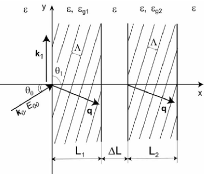
Figure 1: The structure with DEAS in two uniform slanted gratings of widths $L_{1}$ and $L_{2}$ , separated by a gap of width $\Delta L$. The incident rectangular pulse: central frequency $\omega_{0}$, the corresponding wavevector $\mathbf{k}_{0}$, amplitude of the electric field in the pulse $E_{00}$.

Consider an isotropic medium with two slab-like, uniform, holographic grating with sinusoidal modulation of the dielectric permittivity (Fig. 1):

$$\epsilon_{s} = \epsilon+\epsilon_{g1}\exp(\mathrm{i}q_{x}x+\mathrm{i}q_{y}y)+\epsilon_{g1}^{\ast}\exp(-\mathrm{i}q_{x}x-\mathrm{i}q_{y}y)$$

$$\textrm{if}\,\,\,\,0<x<L_{1},$$

$$\epsilon_{s} = \epsilon+\epsilon_{g2}\exp(\mathrm{i}q_{x}x+\mathrm{i}q_{y}y)+\epsilon_{g2}^{\ast}\exp(-\mathrm{i}q_{x}x-\mathrm{i}q_{y}y)$$

$$\textrm{if}\,\,\,\,L_{1}+\Delta L<x<L_{1}+\Delta L+L_{2},$$

$$\epsilon_{s}=\epsilon\,\,\,\,\textrm{elsewhere},$$ (1)

where $L_{1,2}$ are the widths of the two gratings, $\epsilon_{g1,2}$ are the grating amplitudes, $\Delta L$ is the width of the gap between the uniform gratings—see Fig. 1 ($\Delta L$ may be zero, and then we have two joint gratings), the mean dielectric permittivity, $\epsilon$, is the same everywhere in the structure, $q_{x}$ and $q_{y}$ are the $x$- and $y$-components of the reciprocal lattice vector $\mathbf{q}$ that is the same for both the gratings, $q=2\pi/\Lambda$, $\Lambda$ is the period of the gratings, the coordinate system is shown in Fig. 1. The two gratings have different phases: $\phi=\mathrm{arg}(\epsilon_{g2})-\mathrm{arg}(\epsilon_{g1})$ is the phase shift between the gratings. There is no dissipation in the medium ($\epsilon$ is real and positive), and the structure is infinite along the $y$- and $z$-axes.

Non-steady-state DEAS in the this structure occurs when the incident wave is switched on at some moment of time (e.g., at $t=0$). Then, both the incident and scattered wave amplitudes inside and outside the gratings evolve in time and gradually relax to their steady-state values at $t=+\infty$. This occurs when an infinitely long, sinusoidal, step-function incident pulse is switched on at t = 0 at the front grating boundary. The pulse has the amplitude of the electric field $E_{00}$, infinite aperture along the $y$- and $z$-axes, and the angle of incidence $\theta_{0}$ (non-conical geometry—Fig. 1).

However, the numerical analysis of an infinitely long pulse is inconvenient, since its Fourier transform contains a $\delta$-function. Therefore, the method of analysis of non-steady-state EAS, developed in [9], has been based on the consideration of a rectangular sinusoidal incident pulse of finite (rather than infinite) length. The same method is immediately applicable for the approximate and rigorous analyses of DEAS in the considered structures (Fig. 1). In this case, in order to calculate non-steady-state amplitudes of the incident and scattered waves in the structure at an arbitrary moment of time $t=t_{0}$, we consider an incident pulse (Fig. 1) of the time length $2t_{0}$ [9]. Paper [9] also assumed that at $t=0$ the incident pulse was switched on simultaneously (with the amplitude $E_{00}$) everywhere inside the grating and in front of it within the region $L-2t_{0}c^{-1/2}\cos\theta_{0}<x<L$, where $L=L_{1}+\Delta L+L_{2}$. That is, the process of propagation of the pulse through the gratings was ignored (for a detailed justification of this approximation see [9]). In this Letter, we will compare this approximation with the case when the incident wave is switched on at $t=0$ everywhere at the front grating boundary and then propagates through the grating. It is important that both these methods can be equally used for the analysis of non-steady-state DEAS (see below).

The incident rectangular pulse at $t=0$ is expanded into the Fourier integral with respect to time, and its frequency spectrum is determined analytically. As a result, the incident pulse is represented by a superposition of an infinite number of plane waves having different frequencies and amplitudes (determined by the Fourier coefficient in the integral), and the same angle of incidence $\theta_{0}$ (Fig. 1). Each of these plane waves is regarded as an incident plane wave with the determined amplitude at the front grating boundary. Steady-state scattering of these waves is then analyzed by means of the rigorous [4,10] or approximate (if applicable) [1–3] theory of steady-state DEAS.

The rigorous theory [4,10] is based on the enhanced T-matrix algorithm [11,12]. As a result, we obtain steady-state amplitudes of the 0th and $+1$ diffracted orders inside and outside the gratings, corresponding to each of the plane waves in the Fourier spectrum of the incident pulse. Interference of the steady-state $+1$ diffracted orders at the moment of time $t=t_{0}$ (i.e., the inverse Fourier transform applied to these scattered waves) gives the overall (non-steady-state) scattered wave amplitude as a function of the $x$-coordinate [9]. Note that due to the geometry of the problem the non- steady-state incident and scattered wave amplitudes should not depend on the $y$-coordinate. Similarly, applying the inverse Fourier transform to all the 0th diffracted orders in the gratings, gives the overall (non- steady-state) amplitude of the incident pulse in the grating at $t=t_{0}$ as a function of the $x$-coordinate [9] Note that in order to minimize numerical errors [9], the inverse Fourier transform is taken at $t=t_{0}$, i.e., at the middle of the incident pulse. Applying the same procedure for different values of $t_{0}$ (i.e., for incident pulses of different time length $2t_{0}$), we obtain the time evolution of non-steady-state amplitudes of the incident and scattered waves inside and outside the gratings.

Very similarly, for gratings with small amplitude, the approximate theory of steady-state DEAS, based on the allowance for the diffractional divergence of the scattered wave [1–3], can be used instead of the rigorous coupled wave analysis. However, in the case of non-steady-state DEAS, the approximate theory does not lead to simple analytical results (as in papers [1–3]). Therefore, there is little reason to use the approximate approach from the view-point of simplification of the analysis. Nevertheless, the approximate approach of non-steady-state DEAS is important because it is immediately applicable for the analysis of all types of waves in different kinds of periodic gratings with small grating amplitude (e.g., for guided modes in a slab with a corrugated interface—see [2,3,7]).

The described rigorous and approximate theories of non-steady-state DEAS are applicable for all (not only rectangular) shapes of the incident pulse, as well as for an incident beam of finite aperture. However, for beams of finite aperture, we should also use the spatial Fourier analysis.

Due to large time intervals required for the analysis of non-steady-state DEAS, a logarithmic distribution of time points has been used (thus, the fast Fourier transform cannot be used for this analysis). The calculations are carried out separately for each moment of time $t_{0}$. Therefore, there is no accumulation of numerical errors, and noticeable errors at small times $\approx 10^{-13}$s do not affect the accuracy of the results at larger time intervals (see above and [9]).

3 Numerical results

Using the described numerical algorithm, non- steady-state DEAS of bulk TE electromagnetic waves in non-uniform holographic gratings with a phase shift $\phi\neq 0$ has been analysed. The grating parameters are as follows: $\epsilon=5$, $\epsilon_{g1}=|\epsilon_{g2}|=5\times 10^{-3}$, $\theta_{0}=45^{\circ}$, and the wavelength in vacuum (corresponding to the central frequency $\omega_{0}$ of the spectrum of the incident rectangular pulse) $\lambda_{0}=1\mu$m. First, consider the case with $\Delta L=0$ (two joint uniform gratings). We also assume that $L_{1}=L_{2}$ (the effect of non-equal grating widths of the joint gratings on EAS is considered in [2]). The Bragg condition is assumed to be satisfied precisely for the $+1$ diffracted order at $\omega=\omega_{0}$:

$$\mathbf{k}_{1}(\omega_{0})=\mathbf{k}_{0}(\omega_{0})-\mathbf{q}$$ (2)

where $\mathbf{k}_{0}(\omega)$ are the frequency dependent wave vectors of the plane waves in the Fourier integral of the incident pulse, $\mathbf{k}_{1}(\omega)$ are the wave vectors of the corresponding $+1$ diffracted orders (scattered waves), $k_{1}(\omega_{0})=k_{0}(\omega_{0})=\omega_{0}\epsilon^{1/2}/c$ (i.e., the Bragg condition is satisfied for the central frequency $\omega_{0}$), $\mathbf{k}_{1}(\omega_{0})$ is parallel to the grating boundaries (Fig. 1), $c$ is the speed of light. Note that if $\omega\neq\omega_{0}$, $\mathbf{k}_{1}(\omega)$ is not parallel to the grating boundaries [13].

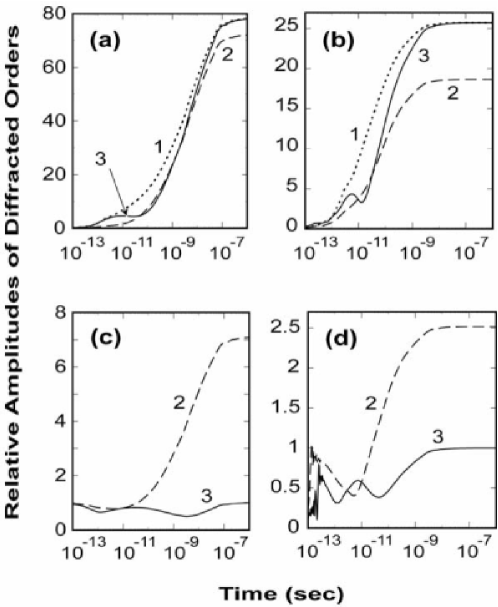
Figure 2: The typical time dependencies of the relative non-steady-state amplitudes of (a), (b) the $+1$ diffracted order (scattered wave) $|E_{1}/E_{00}|$, and (c), (d) the 0th diffracted order (incident wave) $|E_{0}/E_{00}|$ in the holographic gratings with the parameters: $\epsilon=5$, $\epsilon_{g1}=|\epsilon_{g2}|=5\times 10^{-3}$, $\theta_{0}=45^{\circ}$, the vacuum wavelength at $\lambda_{0}=1\mu$, $\Delta L=0$ (joint gratings), at different grating widths: (a), (c) $L_{1}=L_{2}=10\mu$m and $\phi=\mathrm{arg}(\epsilon_{g2}=\phi_{r}\approx 191.2^{\circ}$, (b), (d) $L_{1}=L_{2}=15\mu$m and $\phi=\phi_{r}\approx 205.2^{\circ}$. Dotted curves—front boundary ($x=0$), dashed curves—middle of the grating, i.e., the boundary between the gratings ($x=L_{1}$), solid curves—rear boundary ($x=L_{1}+L_{2}$).

Typical time dependencies of non-steady-state amplitudes of the $+1$ and 0th diffracted orders are presented in Fig. 2(a)–(d) at the resonant phase shifts $\phi=\phi_{r}$ for the two different total grating widths: $L=L_{1}+L_{2}=2L_{1}=20\mu$m ($\phi_{r}\approx 191.2^{\circ}$—Fig. 2(a), (c) and $L=L_{c}\approx 30\mu$m ($\phi_{r}\approx 205.2^{\circ}$—Fig. 2(b), (d); recall that $\Delta L=0$ (joint gratings). The curves in Fig. 2(a), (c) have been calculated under the assumption that the incident wave is switched on simultaneously in the whole grating at $t=0$ (see also [9]), while the curves in Fig. 2(b), (d) have been calculated for the incident wave being switched on at $t=0$ everywhere at the front grating boundary, and then propa- gating through the grating. Both these approximations are equivalent for non-steady-state DEAS (and EAS) at times that are larger than the time that takes for the incident beam to cross the grating. It can be seen that these approximations give different results only for the incident wave amplitude (compare Fig. 2(c) and (d)) and only at small time intervals ($\leq 4\times 10^{-13}$s). Fast oscillations of the curves in Fig. 2(d) within these time intervals are associated with the computational errors related to poor convergence of the Fourier integral near the front end of the rectangular incident beam (as it propagates through the grating). The sharp jumps of the curves in Fig. 2(d) indicate the front end of the incident beam passing through the middle of the grating (dashed curve in Fig. 2(d)) and rear boundary (solid curve in Fig. 2(d)). Note again that the mentioned errors do not affect the results at larger times after the front end of the incident beam has passed through the grating. The effect of propagation of the front end of the incident beam through the grating on the non-steady-state scattered wave amplitudes is completely negligible, because the scattered wave amplitudes within these time intervals are close to zero (Fig. 2(b)).

One of the main results that can be derived from Fig. 2(a)–(d) is the relaxation times for the steady-state regime of DEAS in the considered gratings. It can be seen that for all the curves in Fig. 2(a), (c) the relaxation time is about $\tau\approx 6\times 10^{-9}$s. Within this time interval, the scattered wave will propagate along the grating the distance $\tau c\epsilon^{-1/2}\approx 80$ cm. Taking into account the angle of incidence $\theta_{0}=45^{\circ}$, this distance gives the critical aperture of the incident beam $l_{c}\approx\tau c\epsilon^{-1/2}\cos(\theta_{0})\approx 57$ cm. Only if the aperture of the incident beam is larger that the critical aperture $l_{c}$, can the steady-state regime of DEAS be achieved in the structure. It is obvious that for the considered structure, the steady-state regime of DEAS is difficult to achieve, since this would require excessively wide coherent incident beams and, which is even more problematic, a very long (longer than 80 cm) grating.

Therefore, we have considered non-steady-state DEAS in a wider grating of $L=L_{c}\approx 30\mu$m ($\Delta L=0$ and $L_{1}=L_{2}$ )—Fig. 2(b), (d). In this case, as demon- strated by Fig. 2(b), the relaxation time for the front grating boundary is $\tau\approx 5\times 10^{-11}$s, while in the middle of the grating and at its rear boundary $\tau\approx 2\times 10^{-10}$s. These relaxation times give the critical apertures of the incident beam of $\approx 0.5$ and $\approx 2$ cm, respectively. These apertures (and thus the lengths of the grating) are quite reasonable and easy to achieve in practice.

Another interesting feature that can be seen from Fig. 2(a), (b) is that the relaxation at the front grating boundary (dotted curves) occurs smoothly without any noticeable bumps or minimums, whereas in the middle of the grating and at its rear boundary the time dependencies of the scattered and incident wave amplitudes are characterised by a non-monotonic behaviour (Fig. 2(a)–(d)). This suggests that the non-steady-state $x$-dependencies of the incident and scattered waves inside the grating should be non-symmetrical with respect to the middle of the grating. This is indeed demonstrated by Fig. 3(a), (b).

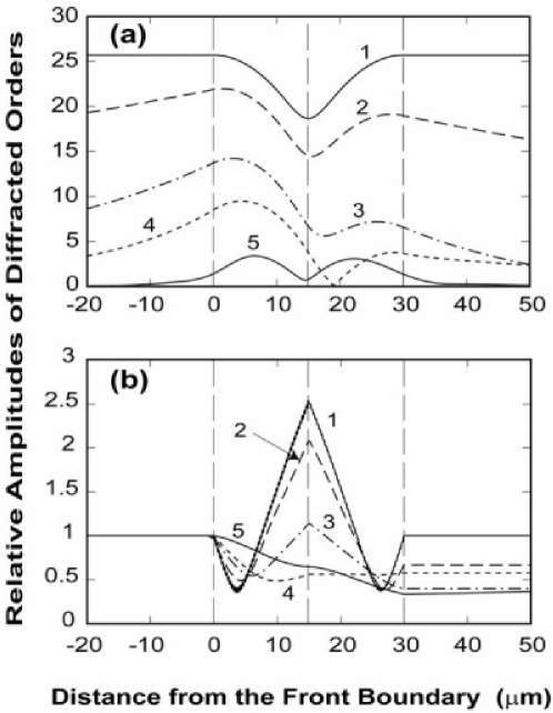
Figure 3: The dependencies of the relative scattered (a) and incident (b) wave amplitudes inside and outside the two joint grating with DEAS on distance from the front grating boundary at different moments of time after switching the incident pulse on: (1) $t=\infty$ (steady-state DEAS), (2) $t=5\times 10^{-10}$s, (3) $t=5\times 10^{-11}$s, (4) $t=10^{-11}$s, (5) $t=10^{-12}$s. The structure is the same as for Fig. 2(b), (d): $\epsilon=5$, $\epsilon_{g1}=|\epsilon_{g2}|=5\times 10^{-3}$, $\theta_{0}=45^{\circ}$, $\lambda_{0}=1\mu$, $\Delta L=0$, $L_{1}=L_{2}=15\mu$, $\phi=\phi_{r}\approx 205.2^{\circ}$. The vertical dashed lines represent the grating boundaries.

Curves 1 in Fig. 3(a), (b) represent the $x$-dependencies of scattered (Fig. 3(a)) and incident (Fig. 3(b)) wave amplitudes for steady-state DEAS (see also [1,2,4]) in the same structure as was used for Fig. 2(b), (d). In particular, it can be seen that at small time intervals (strongly non-steady-state DEAS) the amplitude of the $x$-dependent scattered wave amplitude is characterised by two distinct maximums in the middle of each of the joint gratings (curve 5 in Fig. 3(a)). This is expected because of the following reasons. Within small time intervals (that are nevertheless larger than the time for the incident pulse to cross the grating) the amplitude of the incident wave is practically the same in both the gratings (rescattering of a weak scattered wave can hardly affect the amplitude of the incident wave anywhere in the grating). Therefore, scattering of this incident wave in both the joint gratings results in the same amplitudes of the scattered waves. This is the reason that there are two maxima on curve 5 in Fig. 3(a), approximately of the same height. At the same time, due to the phase shift between the joint gratings ($\phi=\phi_{r}\approx\pi$), the scattered waves in these gratings will approximately be in antiphase with each other. This is the reason that the scattered wave amplitude is approximately zero at the boundary between the gratings (curve 5 in Fig. 3(a)).

With increase of time, the scattered waves start diverging from one grating into another, and this leads to the interaction between the joint gratings. As a result, the minimum of the scattered wave amplitude at the boundary between the gratings shifts to the right (into the second grating), resulting in non-symmetric dependencies (curves 2–4 in Fig. 3(a)). Due to this process, both the amplitudes of the scattered and incident waves in the grating increase, resulting in a strong DEAS resonance (curves 1 in Fig. 3(a), (b)). It is also interesting that once the maximum of the incident wave amplitude in the middle of the grating is established, it does not move anywhere from the boundary between the gratings with increasing time, but just increases in height—see curves 1–4 in Fig. 3(b). For more detailed discussion of physical reasons for DEAS in the considered structure see [1,2].

It is also important to stress out again that for the considered structures the approximate [1,2] and rigorous [4] theories of steady-state DEAS give approximately the same results (with the accuracy of $\approx 7$% for Fig. 2(a), (c) and $\approx 1$% for Figs. 2(b), (d) and 3(a), (b) [4]). Therefore, the presented dependencies in Figs. 2 and 3 can simultaneously be regarded as approximate and rigorous. The agreement between the approximate and rigorous theories generally improves with decreasing time intervals after switching the incident wave on. This is because at smaller time intervals the scattered wave amplitudes are smaller, which makes it easier to satisfy the applicability conditions for the approximate theory (see [10,14]).

Previously [3], it has been demonstrated that strong DEAS resonance can occur not only in two joint gratings with a resonant phase shift, but also in two uniform gratings separated by a gap of width $\Delta L\neq 0$ (Fig. 1). In this case, DEAS occurs due to diffractional divergence of the scattered waves from one of the gratings into another across the gap [3] (the mean permittivity was regarded to be the same throughout the structure).

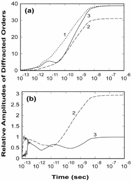
Figure 4: The typical time dependencies of the relative non-steady-state amplitudes of (a) the $+1$ diffracted order (scattered wave) $|E_{1}/E_{00}|$, and (b) the 0th diffracted order (incident wave) $|E_{0}/E_{00}|$ for DEAS in the two separated gratings with the parameters: $\epsilon=5$, $\epsilon_{g1}=|\epsilon_{g2}|=5\times 10^{-3}$, $\theta_{0}=45^{\circ}$, $\lambda_{0}=1\mu$, $\Delta L=10\mu$m (separated gratings), $L_{1}=L_{2}=10\mu$, and $\phi=\phi_{r}\approx 213^{\circ}$. Dotted curve—front boundary ($x=0$), dashed curves—middle of the gap ($x=L_{1}+\Delta L/2=15\mu$m), solid curves—rear boundary ($x=2L_{1}+\Delta L=30\mu$m).

The typical time dependencies of non-steady-state amplitudes of the scattered and incident waves in the middle of the gap (i.e., at $x=L_{1}+\Delta L/2$) and at the front and rear boundaries of the structure (i.e., at $x=0$ and $x=2L_{1}+\Delta L$—Fig. 1) are presented in Fig. 4(a), (b). Here, we again assume equal widths of the interacting gratings ($L_{1}=L_{2}=10\mu$m). It can be seen that there no significant differences between Figs. 4(a), (b) and 2(a)–(d) (except for the lower resonance in Fig. 4(a), (b) compared to that in the same structure but without the gap–Fig. 2(a), (c)). This clearly confirms that the physical reasons behind DEAS in joint and separated gratings are the same—interaction between the gratings by means of the diffractional divergence of the scattered wave from one of the gratings into another [1–3].

The approximation with the incident pulse being switched on everywhere at the front grating boundary at $t=0$ has been used for Fig. 4(a), (b). This is the reason for seeing the effects of propagation of the incident wave through the grating at small time intervals in Fig. 4(b) (similar to those in Fig. 2(d)).

The relaxation times for the front boundary ($x=0$), middle of the gap ($x=L_{1}+\Delta L/2$), and rear boundary ($x=2L_{1}+\Delta L$) are $\tau\approx 3\times 10^{-10}$s, $\tau\approx 6\times 10^{-10}$s, and $\tau\approx 7\times 10^{-10}$s, respectively. These times correspond to the critical apertures of the incident beam $\approx 3$, $\approx 6$, and $\approx 7$ cm, respectively. Increasing gap width between the gratings results in reducing the height and sharpness of the DEAS resonance. This is because the interaction between the gratings by means of diffractional divergence becomes less efficient with increasing gap width, since the scattered waves must be spread by diffractional divergence across a larger distance (for more detailed discussion see [3]). As a result, increasing gap width results in decreasing relaxation times in the gratings and the gap. Conversely, decreasing gap width results in a rapid increase of height and sharpness of the DEAS resonance [1–3]. Thus the relaxation times in this case quickly increase, making such a resonance difficult to achieve in practice (see the comments for Fig. 2(a), (c)).

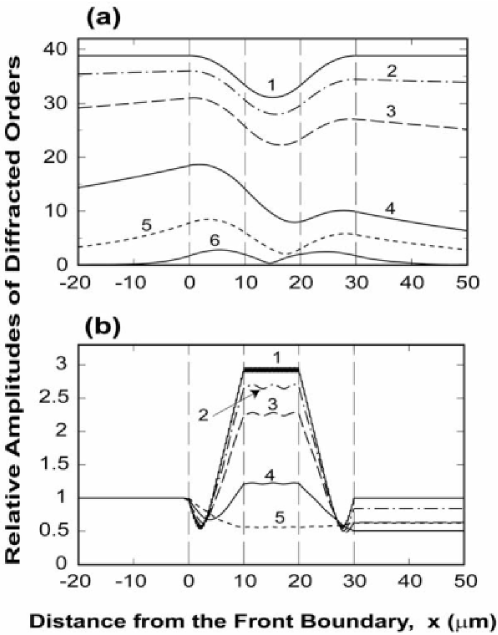
Figure 5: The $x$-dependencies of the relative scattered (a) and incident (b) wave amplitudes inside and outside the two separated grating with DEAS at different moments of time: (1) $t=\infty$ (steady-state DEAS), (2) $t=5\times 10^{-9}$s, (3) $t=10^{-9}$s, (4) $t=10^{-10}$s, (5) $t=10^{-11}$s, (6) $t=10^{-12}$s. The structure is the same as for Fig. 4: $\epsilon=5$, $\epsilon_{g1}=|\epsilon_{g2}|=5\times 10^{-3}$, $\theta_{0}=45^{\circ}$, $\lambda_{0}=1\mu$, $\Delta L=10\mu$m (separated gratings), $L_{1}=L_{2}=10\mu$, and $\phi=\phi_{r}\approx 213^{\circ}$. The vertical dashed lines represent the grating boundaries.

The rigorous $x$-dependencies of non-steady-state amplitudes of the scattered and incident waves in the two gratings separated by a gap are presented in Fig. 5(a), (b). In this case, at small time intervals, the scattered wave amplitude is next to zero in the middle of the gap (see curve 6 in Fig. 5(a)). This is again expected, since the scattered waves with almost opposite phases (due to $\phi=\phi_{r}\approx\pi$) diverge almost symmetrically from the two gratings and practically cancel each other in the middle of the gap. Further increase of time results in the development of a more complex pattern of interaction of the diverged waves (that are not exactly in antiphase: $\phi_{r}\approx 213^{\circ}$), eventually resulting in steady-state DEAS in the considered structure (curves 1 in Fig. 5(a), (b)).

The incident wave amplitude in the gap is constant on average, but experiences small fast oscillations (with the period of $\approx 0.3\mu$m—curve 1 in Fig. 5(b)). As has been demonstrated in [10], these oscillations are due to interference of the incident wave transmitted through the first grating with waves resulting from boundary scattering of the scattered wave at the boundaries of the second grating. This effect is the result of the rigorous theory of analysis of DEAS. In the approximate theory, there is no boundary scattering, and the amplitude of the incident wave in the gap is constant [3]. Note that the discussed fast oscillations can clearly be seen only on curve 1 for steady-state DEAS. On the other hand, curves 2–5 display sinusoidal behaviour in the gap with much larger spatial period (Fig. 5(b)). These oscillations in fact must have the same period as those in curve 1; the apparent longer period results from undersampling and aliasing (i.e., insufficient number of points along the $x$-axis). Note that the curves in Fig. 5(a) are free from these computational errors, because they do not contain fast oscillations that have to be resolved. A similar (but less obvious) problem also occurred in Fig. 3(b) (compare curve 1 with small and fast oscillations and curves 2–5 where these oscillations are not resolved–Fig. 3(b)).

As has been mentioned above, if we disregard the small and fast oscillations of the curves in Figs. 3(b) and 5(b), the presented time and coordinate dependencies in Figs. 2–5 can equally be regarded as rigorous and approximate (this is the case for gratings with sufficiently small amplitude [10,14]). On the other hand, the approximate theory of steady-state DEAS is immediately applicable for the analysis of scattering of any types of waves (including bulk, guided and surface optical and acoustic waves) in various kinds of periodic gratings (e.g., periodic groove arrays for guided and surface waves) [5,7,8,15]. Therefore, the presented dependencies in Figs. 2–5 are also typical for non-steady-state DEAS of any waves in gratings with phase variations and sufficiently small amplitudes.

The procedure of correlating the obtained dependencies in Figs. 2–5 to the case of non-steady-state DEAS of arbitrarily polarised guided slab modes in a non-uniform periodic groove array is exactly the same as that developed in [15] for steady-state EAS. Obviously, if the grating amplitudes are large, then such a simple correlation is no longer valid, and rigorous theories for each type of waves and periodic gratings should be developed.

4 Conclusions

This Letter has carried out a detailed analysis of non-steady-state DEAS in joint and separated gratings by means of rigorous and approximate algorithms based on the Fourier analysis of the incident pulse and rigorous and approximate theories of steady-state DEAS [1–4]. The main attention has been paid to the investigation of non-steady-state DEAS of bulk TE electromagnetic waves in holographic gratings with step-like variations of phase. However, the obtained results are directly applicable for all types of waves in different kinds of periodic gratings with small periodic modulation of structural parameters. This statement is based on the universal applicability of the approximate theory of steady-state DEAS in gratings with sufficiently small amplitude [1–3].

Typical relaxation times have been calculated for several typical joint and separated gratings. The corresponding critical apertures of the incident beam, that are required for achieving steady-state DEAS, have also been determined. In particular, it has been shown that if the grating width is noticeably smaller than the critical width [1,2], i.e., the DEAS resonance is sufficiently strong, the relaxation time and the corresponding critical aperture of the incident pulse can be too large for this resonance to be achieved in practice. At the same time, increasing grating width and/or introducing a gap between the interacting gratings (separated gratings) results in a quick reduction of height and sharpness of the predicted resonance, and thus the calculated relaxation times and critical apertures of the incident beam. Typical structures that are reasonable for practical observation of DEAS are thus identified.

References

1. D.K. Gramotnev, D.F.P. Pile, Phys. Lett. A 253 (1999) 309.

2. D.K. Gramotnev, D.F.P. Pile, Opt. Quantum Electron. 32 (2000) 1097.

3. D.K. Gramotnev, T.A. Nieminen, Opt. Quantum Electron. 33 (2001) 1.

4. T.A. Nieminen, D.K. Gramotnev, unpublished.

5. M.P. Bakhturin, L.A. Chernozatonskii, D.K. Gramotnev, Appl. Opt. 34 (1995) 2692.

6. D.K. Gramotnev, J. Phys. D 30 (1997) 2056.

7. D.K. Gramotnev, Opt. Lett. 22 (1997) 1053.

8. D.K. Gramotnev, Phys. Lett. A 200 (1995) 184.

9. T.A. Nieminen, D.K. Gramotnev, Opt. Express 10 (2002) 268.

10. T.A. Nieminen, D.K. Gramotnev, Opt. Commun. 189 (2001) 175.

11. M.G. Moharam, E.B. Grann, D.A. Pommet, T.K. Gaylord, J. Opt. Soc. Am. A12 (1995) 1068.

12. M.G. Moharam, D.A. Pommet, E.B. Grann, T.K. Gaylord, J. Opt. Soc. Am. A12 (1995) 1077.

13. D.K. Gramotnev, Frequency response of extremely asymmetrical scattering of electromagnetic waves in periodic gratings, in: 2000 Diffractive Optics and Micro-Optics (DOMO-2000), Quebec City, Canada, 2000, p. 165.

14. D.K. Gramotnev, Opt. Quantum Electron. 33 (2001) 253.

15. D.K. Gramotnev, T.A. Nieminen, T.A. Hopper, J. Mod. Opt. 49 (2002) 1567