Preprint of:
T. A. Nieminen and D. K. Gramotnev
“Rigorous analysis of extremely asymmetrical scattering of electromagnetic waves in slanted periodic gratings”
Optics Communications 189, 175–186 (2003)

1 Introduction

Scattering of bulk and guided electromagnetic waves in periodic gratings has been extensively investigated theoretically and numerically by many different authors using approximate and rigorous methods of analysis [1–17]. The investigation has been carried out for thin and thick, uniform and non-uniform, isotropic and anisotropic, reflecting and transmitting gratings that are represented by strong or weak periodic modulation of structural parameters [1–17].

Very interesting physical effects and anomalies of scattering have been predicted and observed at extreme angles of scattering, i.e., when the scattered wave propagates parallel to the grating. For example, these are resonant coupling of bulk and surface [16,19], or bulk and guided waves [20], non-linear stimulated scattering involving interaction of bulk and surface waves [21–23], Wood’s anomalies [16,17], etc. However, all these effects and anomalies are relevant to scattering in thin gratings, where the incident wave and/or scattered wave interact with the grating within a short distance of the order of, or less than the wavelength [16–23]. For example, this happens in the case of diffraction of a bulk electromagnetic wave on a periodic corrugation of an interface between two media.

Bragg scattering in wide, oblique, periodic gratings with the scattered wave propagating parallel to grating boundaries has been investigated less extensively compared to thin gratings. In the beginning of 1970s a radically new type of Bragg scattering of X-rays in crystals and crystal plates (i.e. thick gratings) was analysed theoretically [24–27]. It was called extremely asymmetrical scattering (EAS). However, the main efforts in theoretical and experimental investigation of EAS of X-ray and neutrons were focused on the cases where an incident wave propagates almost parallel to the front boundary of a crystal [28]. This allowed very precise structural analysis of interfaces and ultra-thin crystal films, and resulted in the development of efficient collimators of X-rays and neutron beams [28]. At the same time, the geometry of EAS with grazing incident wave is not that interesting for the development of applications in optical communication and instrumentation. Much more important is the geometry where the incident wave propagates at a significant angle with respect to boundaries of a strip-like oblique periodic grating, and the scattered wave is parallel or almost parallel to these boundaries. This is because of unique features displayed by EAS in this geometry [29–37]. However, theoretical analysis of EAS of bulk and guided optical and surface acoustic waves has been carried out only within the last few years [29–37].

The diffractional divergence of the scattered wave inside and outside the grating has been shown to be the main physical reason for EAS [29–31,33,34]. A new powerful approach for the analytical analysis of EAS, based on understanding the role of the diffractional divergence, has been developed and justified [29–31,33,34]. The most important feature of this approach is that it is immediately applicable for the description of EAS of all types of waves (including bulk, guided and surface optical and acoustic waves) in all types of periodic gratings with small amplitude [29–37].

It has been shown that EAS is characterised by a resonantly large scattered wave amplitude (the most interesting case of scattering) only if the grating amplitude is very small [29–34]. In this case, the applicability conditions for the new approach are usually well satisfied [37], and the analytical theory is expected to be accurate in predicting amplitudes of the incident and especially scattered waves.

Since the main direction in the development of the modern theory of gratings is related to improvement of stability and convergence speed of numerical algorithms (see for example Ref. [9]), the development of the new numerically efficient (analytical) method for the accurate description of strong EAS (of all types of waves, including guided and surface modes) is an important step in the grating theory. Moreover, this method has provided a unique insight into the physical reasons for EAS [29–37]. This insight will allow thoughtful selection of optimal structural parameters for future EAS-based devices and techniques.

Nevertheless, despite the fact that the new analytical approach is expected to describe accurately EAS with strong resonant increase of the scattered wave amplitude, it is still unknown what happens to EAS beyond the frames of the applicability of the analytical approach. That is, what changes in the pattern of scattering should be introduced if the grating amplitude is strongly increased and/or grating width is significantly reduced? What are the exact errors of using the analytical approach for various grating amplitudes and widths? How accurate are the applicability conditions for the approximate theory? What are the most crucial parameters affecting the applicability of the analytical approach? Which of the two waves—incident or scattered—is better described by the approximate theory? All these questions remained largely unanswered in the previous publications.

Therefore, the main aim of this paper is to implement detailed rigorous analysis of EAS of bulk TE electromagnetic waves in narrow and wide periodic gratings of arbitrary amplitude, represented by sinusoidal variations of the dielectric permittivity. In addition, the analytical applicability conditions for the approximate theory of EAS will be verified and compared with the results of the rigorous theory. Physical mechanisms that are responsible for breaching these conditions will be discussed. Typical errors related to the approximations of the analytical approach will be determined.

2 Numerical analysis

Consider an isotropic medium with a slab-like holographic periodic grating that is characterised by sinusoidal variations of the dielectric permittivity:

$$\epsilon_{s} = \epsilon+(\epsilon_{1}\exp(\mathrm{i}q_{x}x+\mathrm{i}q_{y}y)+\textrm{c.c.}),\,\,\,\,\textrm{if }0<x<L,$$

$$\epsilon_{s} = \epsilon,\,\,\,\,\textrm{if }x<0\textrm{ or }x>L.$$ (1)

where the coordinate system is shown in Fig. 1, $\epsilon$ is the mean dielectric permittivity that is the same inside and outside the grating, $\epsilon_{1}$ is the complex amplitude, $\mathbf{q}=(q_{x},q_{y})$ is the reciprocal lattice vector, $q=2\pi/\Lambda$, $\Lambda$ is the period, and $L$ is the width of the grating that is assumed to be infinite along the $y$- and $z$-axes. We also assume that the dissipation is absent, i.e., $\epsilon$ is real and positive. A TE electromagnetic wave with the amplitude $E_{00}$ and wave vector $\mathbf{k}_{0}$ is incident onto the grating at an angle $\theta_{0}$ in the $xy$ plane—Fig. 1 (non-conical scattering).

Figure 1: The geometry of EAS in a slanted periodic grating of width $L$. The Bragg condition is satisfied precisely for the $+1$ harmonic that propagates parallel to the grating boundaries $x=0$ and $x=L$. The angle of incidence $\theta_{0}$ is not close to $\pi/2$.

In this case the solutions inside and outside the grating can be written as [7,8]

$$E(x,y)=\sum_{h=-\infty}^{+\infty}E_{h}(x)\exp(\mathrm{i}xk_{hx}+\mathrm{i}yk_{hy}),$$ (2)

$$E|_{x<0}=E_{00}\exp(\mathrm{i}\mathbf{k}_{0}\cdot\mathbf{r})+\sum_{h=-\infty}^{+\infty}A_{h}\exp((\mathrm{i}\mathbf{k}_{1h}\cdot\mathbf{r}),$$ (3)

$$E|_{x>L}=\sum_{h=-\infty}^{+\infty}B_{h}\exp(\mathrm{i}\mathbf{k}_{2h}\cdot\mathbf{r}-\mathrm{i}Lk_{2hx}),$$ (4)

where $k_{hx}$ and $k_{hy}$ are the $x$- and $y$-components of the wave vectors

$$\mathbf{k}_{h}=\mathbf{k}_{0}-h\mathbf{q}\,\,\,\,(h=0;\pm 1,\pm 2,...),$$ (5)

the components of the wave vectors k1 h and k2 h are determined by the equations:

$$k_{1hy}=k_{2hy}=k_{hy},\,\,\,\,k_{1hx}=-k_{2hx}=-(k_{0}^{2}-k_{hy}^{2})^{1/2}.$$ (6)

If $k_{hy}\leq k_{0}$, then $k_{1hx}\leq 0$ and $k_{2hx}\geq 0$ (propagating waves), while if $k_{hy}>k_{0}$, then $\mathrm{Im}(k_{1hx})<0$ and $\mathrm{Im}(k_{2hx})>0$ (evanescent waves).

The Bragg condition is assumed to be satisfied precisely for the $+1$ harmonic in Eq. (2), i.e. for the first diffraction order with $h=1$. In addition, the $+1$ harmonic is assumed to propagate parallel to the $x$-axis (the geometry of EAS).

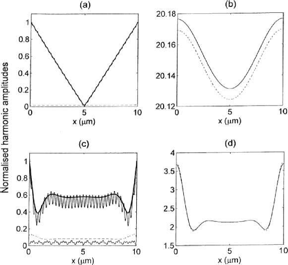
Figure 2: The $x$-dependencies of the normalised amplitudes $|E_{h}/E_{00}|$ of harmonics in Eq. (2) inside the grating with the parameters: $\epsilon=5$, $\theta_{0}=45^{\circ}$, $L=10\mu$, $\lambda=1\mu$ (in vacuum), and with the grating amplitudes: (a,b) $\epsilon_{1}=5\times 10^{-3}$, (c,d) $\epsilon_{1}=0.2$. The grating orientation and period $\Lambda\approx 0.584\mu$m are determined by the Bragg condition. (a) The rigorous (solid curve with small oscillations) and approximate (solid curve without oscillations) $x$-dependencies of the amplitude of the zeroth harmonic (incident wave) inside the grating. Dotted curve—the rigorous $x$-dependence of the $+2$ harmonic amplitude. (b,d) The rigorous (dotted curves) and approximate (solid curves) dependencies of amplitudes of the $+1$ harmonics (the scattered waves) inside the grating. (c) The thick solid curve is the approximate $x$-dependence of the amplitude of the incident wave inside the grating. The rigorous $x$-dependencies of amplitudes of the 0th, $+2$, and $-1$ harmonics are presented by the higher thin solid curve, dotted curve, and lower thin solid curve, respectively.

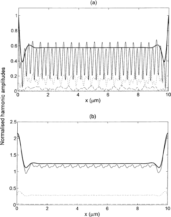
Figure 3: The rigorously calculated $x$-dependencies of the normalised amplitudes $|E_{h}/E_{00}|$ of harmonics in Eq. (2) in the same structure as for Fig. 2, but with $\epsilon_{1}=1$. (a) The rigorous dependencies of amplitudes of the 0th harmonic (thin solid curve), $-1$ harmonic (higher dotted curve), $-2$ harmonic (dashed curve), and $-3$ harmonic (lower dotted curve). (b) The rigorous dependencies of amplitudes of the $+1$ harmonic (thin solid curve), $+2$ harmonic (dotted curve), and $+3$ harmonic (dashed curve). The thick solid curves represent the approximate $x$-dependencies of the incident (a) and scattered (b) wave amplitudes, obtained from the approximate theory [29–32].

The rigorous analysis of first-order scattering in this geometry has been carried out by means of the enhanced transmittance matrix algorithm [7]. Fig. 2 presents the approximate and rigorous $x$-dependencies of normalised amplitudes of harmonics from Eq. (2) inside the grating for EAS of bulk TE electromagnetic waves. The structural parameters are as follows: $\epsilon=5$, $\theta_{0}=\pi/4$, $L=10\mu$m, vacuum wavelength $\lambda=1\mu$m, and the grating amplitudes are $\epsilon_{1}=5\times 10^{-3}$ (Fig. 2a and b) and $\epsilon_{1}=0.2$ (Fig. 2c and d). The grating period is determined by the Bragg condition: $\Lambda\approx 0.584\mu$m. Similar dependencies in Fig. 3a and b are presented for the same structure but with the grating amplitude $\epsilon_{1}=0.2$. Only harmonics whose amplitudes are larger than $\approx 0.01E_{00}$ are presented in Figs. 2 and 3.

It can be seen that in gratings with small amplitudes, where the scattered wave amplitude is especially large (Fig. 2a and b), the eect of all harmonics in the expansion (2), other than the zeroth harmonic (the incident wave) and the $+1$ harmonic (the scattered wave), is completely negligible. The rigorous $x$-dependencies of the incident and scattered wave amplitudes inside the grating hardly dier from the corresponding approximate dependencies that have been determined by means of the approximate theory [31] (Fig. 2a and b). Thus, for sufficiently small grating amplitudes the approximate theory [29–34] provides a very accurate description of EAS and there is no need for the rigorous analysis. The only other harmonic (in addition to the zeroth and $+1$ harmonics) that may have reasonably noticeable amplitude is the $+2$ harmonic. This is due to the direct coupling of the resonantly strong scattered wave (the $+1$ harmonic) and the $+2$ harmonics [4].

However, if the grating amplitude is significantly increased from $5\times 10^{-3}$ to $0.2$ (Fig. 2c and d) and then to 1 (Fig. 3a and b), then the approximate theory is not always sufficient for the description of EAS. This is especially the case for the amplitude of the incident wave, i.e. the zeroth harmonic in Eq. (2). For example, if $\epsilon_{1}=0.2$ (Fig. 2c), then the rigorously calculated $x$-dependence of the zeroth harmonic amplitude is noticeably lower (on average) than the corresponding approximate dependence (Fig. 2c), and is characterised by a number of oscillations (see also Fig. 3a).

These oscillations are related to boundary scattering of the scattered wave at the grating interface $x=L$. The wave resulting from boundary scattering of the scattered wave at the rear boundary $x=L$ propagates in the negative $x$-direction as if it is a mirror reflected incident wave from this boundary. Thus, the $y$-component of its wave vector is equal to the $y$-component of the wave vector of the incident wave. However, the wave due to boundary scattering is not presented explicitly in Eq. (2). Therefore the zeroth harmonic in Eq. (2) includes both the incident wave and the wave caused by boundary scattering at $x=L$. The interference of these waves results in a standing wave pattern represented by the fast oscillations of the zeroth harmonic amplitude—Figs. 2c and 3a. It can be seen that the period of this standing wave pattern must be equal to $\lambda/(2\epsilon^{1/2}\cos\theta_{0})$, which is in the excellent agreement with the rigorous dependencies in Figs. 2c and 3a.

As mentioned above, the average (over the period $\lambda/(2\epsilon^{1/2}\cos\theta_{0})$) rigorously calculated amplitude of the zeroth harmonic tends to be smaller than the amplitude predicted by the approximate theory—see Figs. 2c and 3a. The larger the grating amplitude, the smaller the average amplitude of the zeroth harmonic inside the grating (Figs. 2c and 3a). This is related to significant boundary scattering at the front grating interface, which results in energy losses in the zeroth harmonic with subsequent reduction of its amplitude in the grating.

The contribution of higher harmonics to scattering rapidly increases when the grating amplitude $\epsilon_{1}$ exceeds $\approx 10$% of the mean permittivity $\epsilon$ (compare Figs. 2c and 3a,b). It is however important that amplitude of the scattered wave is accurately described by the approximate theory (within an error less than $\approx 1$%) up to grating amplitudes such that $\epsilon_{1}/\epsilon\approx 0.1$. Only when $\epsilon_{1}/\epsilon=0.2$ can noticeable deviations between the rigorous and approximate amplitudes of the $+1$ harmonic be observed (Fig. 3a and b).

Increasing grating amplitude should result not only in noticeable amplitudes of several harmonics in Eq. (2) (see Figs. 2 and 3), but also in significant energy flows from the grating due to propagating waves in Eqs. (3) and (4) (in the considered examples these will correspond to $h=-1,..,-5$). In addition, the zeroth harmonic in the sum of Eq. (3), caused by boundary scattering at the grating interfaces, also results in an energy flow away from the grating in the region $x<0$. The associated energy losses can be evaluated in terms of diffraction efficiencies that are determined as ratios of the $x$-component of the Poynting vector in a wave travelling away from the grating to the $x$-component of the Poynting vector in the incident wave at $x<0$. If the diffraction efficiencies are small compared to one, the energy losses are negligible, and the approximate theory of EAS is valid.

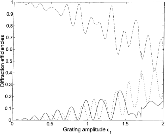
Figure 4: The dependencies of the diffraction efficiencies on grating amplitude $\epsilon_{1}$ for the transmitted wave with the amplitude $B_{0}$ (dashed curve), zeroth reflected wave with the amplitude $A_{0}$ (solid curve), and the combined efficiency for all other propagating waves outside the grating (dotted curve). The other structural parameters are as for the previous figures: $\epsilon=5$, $\theta_{0}=\pi/4$, $L=10\mu$m, $\lambda=1\mu$m, and $\Lambda\approx 0.584\mu$m.

The dependencies of the diffraction efficiencies in the structure with $\epsilon=5$, $\theta_{0}=\pi/4$, $L=10\mu$m, and $\lambda=1\mu$m on grating amplitude $\epsilon_{1}$ are presented in Fig. 4. The dashed curve represents the diffraction efficiency of the transmitted wave, i.e. the zeroth harmonic in Eq. (4). The solid line gives the diffraction efficiency of the wave resulting from boundary scattering (i.e. the zeroth reflected wave for $x<0$), and the dotted curve gives the overall diffraction efficiency from all other waves propagating outside the grating. Note that the diffraction efficiency for the scattered wave, i.e. the $+1$ harmonic, is zero because it propagates parallel to the grating boundaries in both the regions $x<0$ and $x>L$.

It can be seen that if the grating amplitude $\epsilon_{1}<0.12$ (i.e. $\epsilon_{1}<0.025\epsilon$), then all the diffraction efficiencies other than that of the transmitted wave are less than $\approx 0.01$ and can be neglected. The diffraction efficiency for the transmitted wave in this case is $\approx 1$ (Fig. 4).

It is interesting that all the diffraction efficiencies experience significant oscillations with increasing grating amplitude e1 . This is due to the interference of waves at the grating boundaries. For example, the waves caused by boundary scattering at the front and rear grating boundaries interfere constructively or destructively in the region $x<0$, resulting in the oscillations of the solid curve in Fig. 4.

All these results demonstrate that in the most interesting case of EAS with strong resonant increase of the scattered wave amplitude the approximate theory [29–34] gives very accurate results, especially for the scattered wave amplitude. Only when the grating amplitude increases so that the resonant scattered wave amplitude becomes of the order of $E_{00}$, does the approximate theory fail to accurately predict, first, the incident wave amplitude inside the grating, and only then (if the grating amplitude is increased up to $\approx 0.2\epsilon$) the scattered wave amplitude. Note, however, that this is correct only for gratings of widths that are not much less than the critical grating width $L_{c}$ [34–37]

$$L_{c}\approx(2c/\omega)[2\epsilon^{-1}|A_{1}/(E_{00}\epsilon_{1})|]^{1/2},$$ (7)

where $A_{1}$ is the amplitude of the $+1$ harmonic at the front boundary in a wide grating (with $L>_{L}c$—see Refs. [34–36]).

If the grating width $L$ is decreased below $L_{c}$, then the approximate theory predicts that the scattered wave amplitude inside and outside the grating must increase proportionally to $L^{-1}$ [29–32,37]. In this case, even if the grating amplitude is small, the direct coupling of the scattered wave (the $+1$ harmonic) to the $+2$ harmonics must result in increasing amplitude of the $+2$ harmonic inside the grating. In addition, the wave resulting from boundary scattering (i.e. the zeroth harmonic in the sum in Eq. (3)) must also increase proportionally to the amplitude of the scattered wave, i.e. proportionally to $L^{-1}$. These effects suggest that decreasing grating width will eventually lead to the breach of the applicability of the approximate theory [29–32,37].

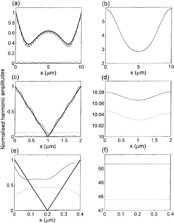
Figure 5: The $x$-dependencies of the normalised amplitudes $|E_{h}/E_{00}|$ of harmonics inside the grating with the parameters: $\epsilon=5$, $\epsilon_{1}=5\times 10^{-2}$, $\theta_{0}=\pi/4$, $\lambda=1\mu$, $\Lambda\approx 0.584\mu$m, and the grating widths: (a,b) $L=10\mu$m, (c,d) $L=2\mu$m, (e,f) $L=0.4\mu$m. (a), (c), and (e) present the rigorous $x$-dependencies of amplitudes of the 0th harmonics (higher thin solid curves), $+2$ harmonics (dotted curves), and $-1$ harmonics (lower thin solid curves). The thick solid curves are the approximate $x$-dependencies of the incident wave amplitudes in the gratings. (b), (d), and (f) present the rigorous (dotted curves) and approximate (solid curves) $x$-dependencies of amplitudes of the $+1$ harmonics (scattered waves).

Fig. 5 presents the results of the rigorous and approximate analyses of EAS in gratings of different widths: (a) and (b) $L=10\mu$m; (c) and (d) $L=2\mu$m; (e) and (f) $L=0.4\mu$m. The other parameters are: $\epsilon=5$, $\epsilon_{1}=5\times 10^{-2}$, $\theta_{0}=\pi/4$, $\lambda=1\mu$.

We can see that for $L=10\mu$ the pattern of scattering is very much the same as in Fig. 2a–d. The incident wave amplitude inside the grating experiences oscillations similar to those in Fig. 2c, but with smaller amplitude (due to smaller $\epsilon_{1}$). The amplitudes of the $+2$ and $-1$ harmonics are small (Fig. 5a), and the approximate and rigorous curves for the scattered wave amplitude are practically indistinguishable—Fig. 5b.

If the grating width is reduced to $2\mu$m (Fig. 5c and d), then the number of oscillations of the rigorous dependence of the incident wave amplitude inside the grating is significantly reduced. This is because fewer nodes of the standing wave pattern can fit across a narrower grating. The amplitude of the $+2$ harmonic is increased $\approx 2$ times compared to the amplitude of the same harmonic in Fig. 5a. This is because the amplitude of the scattered wave in Fig. 5d is $\approx 2$ times larger than in Fig. 5b. Note that for $L=2\mu$m, the rigorous dependence of the $+1$ harmonic amplitude is only $\approx 0.03$% different from the approximate curve (Fig. 5d). That is, the oscillations of the incident wave amplitude and noticeable amplitude of the 2 harmonic (Fig. 5c) hardly affect the scattered wave amplitude.

If the grating width is decreased further down to $0.4\mu$m, then the rigorously calculated dependence of the incident wave amplitude in the grating becomes drastically different from the approximate dependence (Fig. 5e). The amplitude of the $+2$ harmonic becomes large and comparable with the amplitude of the incident wave (Fig. 5e). Note however, that since the $-1$ harmonic is not coupled directly to the resonantly large amplitude of the $+1$ harmonic, the amplitude of the $-1$ harmonic is hardly affected by reducing grating width (compare the lower thin solid curves in Fig. 5a, c, and e).

For the grating width of $0.4\mu$m the $+1$ harmonic amplitude is so large (Fig. 5f), that boundary scattering results in a significant energy flow from the grating. This is the main reason why the rigorously calculated amplitudes of the $+1$ harmonic (scattered wave) appear to be noticeably smaller than those obtained in the approximate theory [31] (Fig. 5f). The difference between these curves is about 5%. Thus, edge effects in the form of boundary scattering are the main reason for the failure of the approximate theory [29–32] to accurately predict scattered wave amplitudes in the case of EAS in narrow gratings.

Note again that all harmonics in Eq. (2), other than the zeroth, $+1$, $+2$, and $-1$ harmonics, have very small amplitudes in the considered structures for all grating widths (Fig. 5a–f), and thus can be neglected.

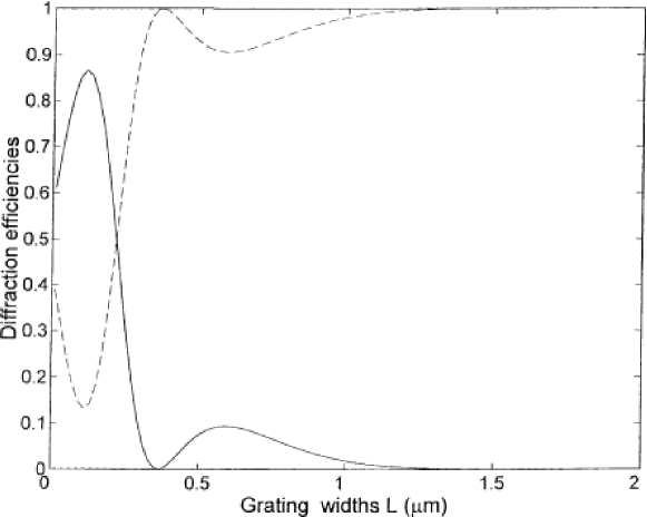
Figure 6: The dependencies of the diffraction efficiencies on grating width $L$ for the transmitted wave with the amplitude $B_{0}$ (dashed curve), zeroth reflected wave with the amplitude $A_{0}$ (solid curve), and the combined efficiency for all other propagating waves outside the grating (dotted curve)—can hardly be seen near the origin of the graph. The structural parameters are the same as for Fig. 5: $\epsilon=5$, $\epsilon_{1}=5\times 10^{-2}$, $\theta_{0}=\pi/4$, $\lambda=1\mu$, and $\Lambda\approx 0.584\mu$m.

The diffraction efficiencies versus grating width for the structure considered for Fig. 5 are presented in Fig. 6. The dashed curve gives the diffraction efficiency of the transmitted wave (the zeroth harmonic at $x>L$), and the solid curve gives the diffraction efficiency for the wave due to boundary scattering. The overall efficiency for other propagating waves is significantly less than 1%, and the relevant dotted curve can hardly be seen close to the origin of the graph (Fig. 6). This figure demonstrates that, as mentioned above, decreasing grating width below $1\mu$m results in significant boundary scattering. This results in the failure of the approximate theory. However, for grating widths $L>1\mu$m all diffraction efficiencies, except for that of the transmitted wave, are negligible (Fig. 6), and the approximate theory gives very accurate results, at least in terms of predicting scattered wave amplitudes inside and outside the grating.

Note that the analysis of the case with $L>L_{c}$ has already been carried out in Figs. 2c,d, 3a,b, and 4. Therefore, increasing grating width beyond $10\mu$m does not reveal any new features of EAS. In addition, the typical number of oscillations of the rigorously calculated dependencies of the wave amplitudes (see Figs. 2, 3, and 5) increases proportionally to $L$, which would make relevant figures unreadable. Therefore, the numerical results have been presented only for gratings of $L\leq 10\mu$m, though the enhanced T-matrix approach is stable for gratings of arbitrary width [7,8].

3 Applicability conditions for the approximate theory

As was demonstrated in the previous section, the approximate theory of EAS, based on the two-wave approximation and the scalar theory of diffraction of the scattered wave [29–32], normally gives accurate results in the most interesting cases of scattering with strong resonant increase of the scattered wave amplitude. It has also been shown [37], that the applicability conditions for the approximate theory of EAS can be evaluated in two different ways. First, we take the applicability condition for the two-wave approximation in the case of the conventional Bragg scattering of TE electromagnetic waves [4]

$$\rho=\lambda^{2}\Lambda^{-2}|\epsilon_{1}|^{-1}=q^{2}\epsilon/(k_{0}^{2}|\epsilon_{1}|)>10$$ (8)

and divide $\rho$ by the normalised maximal value of the scattered wave amplitude:

$$\rho_{\mathrm{EAS}}=\rho|E_{00}/\mathrm{max}(|E_{1}(x)|)|>10$$ (9)

This inequality can be regarded as the applicability condition for the approximate theory of EAS [37]. The factor $|E_{00}/\mathrm{max}(|E_{1}(x)|)|$ appears in inequality (9) because in the case of EAS the scattered wave amplitude is much larger than the amplitude of the incident wave: $|E_{1}|\ll|E_{00}|$. As indicated in Section 2, this may result in unusually strong boundary scattering, oscillations of the incident wave amplitude inside the grating, and large amplitude of the 2 harmonic (all these effects are proportional to $|E_{1}|$).

If inequality (12) is satisfied, then the errors in the energy flux in the scattered wave, which result from the use of the two-wave approximation, are expected to be of the order of $\approx 1/\rho_{\mathrm{EAS}}^{2}$, i.e., less than 1% (see also Ref. [4]).

Another way of evaluating applicability conditions for the approximate theory [29–32,37] is to directly evaluate boundary scattering [37]. Figs. 4 and 6 demonstrate that boundary scattering of a resonantly large scattered wave amplitude is the main source of error in the case of small grating amplitudes. For large grating amplitudes, it gives approximately the same average diffraction efficiency as all other harmonics with $h\neq 0,1$ (Fig. 4). Therefore, conditions for neglecting boundary scattering can be regarded as the applicability conditions for the approximate theory of EAS [29–32,37]. The evaluation of the efficiency of boundary scattering has demonstrated [37] that the energy flow in the zeroth reflected wave at $x<0$ can be neglected if

$$4(\Delta x/L)^{2} \ll 1\,\,\,\,\textrm{if }L\leq L_{c},$$

$$4(\Delta x/L_{c})^{2} \ll 1\,\,\,\,\textrm{if }L>L_{c},$$ (10)

where $L_{c}$ is the critical grating width determined by Eq. (7) [34–37], and $\Delta x$ is the typical thickness of the region around the front grating boundary [37], where from the energy of the scattered wave is transferred into the energy of the boundary scattered wave.

If conditions (10) are satisfied, then the diffraction efficiency for the boundary scattered wave in the region $x<0$ should be of the order of the left-hand sides of inequalities (10) [37]. Knowing these efficiencies, we can easily evaluate typical variations of the scattered wave amplitude inside the grating.

If $L<L_{c}$, then in accordance with condition (10), the diffraction efficiency for the transmitted wave with the amplitude $B_{0}$ (see Eq. (4)) can be evaluated as

$$|B_{0}|^{2}/|E_{00}|^{2}\approx 1-r,$$

where $r=4(\Delta x/L)^{2}$. From this equation we have:

$$|B_{0}|\approx|E_{00}|(1-r/2).$$ (11)

If $L<L_{c}$ , then the approximate theory [29–32] gives that the amplitude of the incident wave inside the grating reduces linearly from the magnitude $|E_{00}|$ to approximately zero in the middle of the grating, and then increases linearly back to $|E_{00}|$—see Figs. 2a, 5c and e. This is due to re-scattering of the scattered wave inside the grating [36,37]. The amplitude of the re-scattered wave increases linearly with increasing $x$ in the grating and has a phase shift $\approx\pi$ with respect to the incident wave. In the middle of the grating, the magnitude of the re-scattered wave amplitude becomes equal to $|E_{00}|$, and at the rear grating boundary $x=L$ it reaches approximately $2|E_{00}|$. If there is noticeable boundary scattering, then the amplitude of the re-scattered wave at the rear boundary is less than $2|E_{00}|$ by the value $\Delta E_{0}\approx r|E_{00}|/2$ (see Eq. (11)). On the other hand, the rate of increasing re-scattered wave amplitude along the $x$-axis is directly proportional to the scattered wave amplitude. Thus we can write:

$$2|E_{00}|-r|E_{00}|/2\approx G|E_{1}|L,$$ (12)

where $G$ is the coefficient of proportionality between $|E_{1}|$ and the rate of increasing re-scattered wave amplitude in the grating. The amplitude of the scattered wave inside the grating is reduced due to energy losses caused by boundary scattering. Thus, $|E_{1}|=|E_{10}|-\Delta E_{1}$, where $E_{10}$ is the scattered wave amplitude determined by means of the approximate theory [29–32], and $\Delta E_{1}$ is the error in the magnitude of this amplitude. Substituting this equation for $|E_{1}|$ in Eq. (12), and taking into account that $A|E_{10}|L\approx 2|E_{00}|$, we obtain:

$$\Delta E_{1}\approx r|E_{00}|/(2AL)\approx 2\Delta x^{2}|E_{00}|/(AL^{3}).$$ (13)

Using Eq. (12) again, we get:

$$\Delta E_{1}/|E_{1}| \approx (\Delta x/L)^{2},\,\,\,\,\textrm{if }L\leq L_{c},$$

$$\Delta E_{1}/|E_{1}| \approx (\Delta x/L_{c})^{2},\,\,\,\,\textrm{if }L>L_{c},$$ (14)

It is obvious that $\Delta x$ should be of the order of, or less than one wavelength in the medium. More accurate evaluation of the thickness $\Delta x$ can be obtained from the comparison of conditions (14) with the rigorous numerical results.

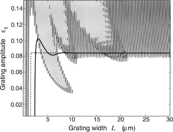
Figure 7: The rigorously calculated contours of 1% difference between the approximate and rigorous scattered wave amplitudes. In the shaded regions, the maximal error in the approximate scattered wave amplitude are larger than 1%, whereas in the unshaded regions this error are less than 1%. The dashed rectangle is the approximate contour of 1% error in the scattered wave amplitude, determined by Eqs. (14) with $\Delta x\approx\lambda_{m}/\mathrm{e}$. Inside this rectangle, the error in the approximate scattered wave amplitude is expected to be smaller than 1%. The thick solid curve represents the approximate contour of 1% error in the scattered wave amplitude, determined from Eq. (15).

Fig. 7 presents the contour plot for the 1% error in the approximate scattered wave amplitude [31] as a function of grating width L and grating amplitude $\epsilon_{1}$ for EAS of bulk TE electromagnetic waves. The structural parameters are as previously: $\epsilon=5$, $\theta_{0}=\pi/4$, $\lambda=1\mu$, and $\Lambda\approx 0.584\mu$m. In the shaded regions the maximal difference (error) between the rigorous and approximate $x$-dependencies of the scattered wave amplitude is more than 1%, while in the unshaded regions this error is less than 1%.

If we assume that in Eqs. (14) $\Delta x=\lambda_{m}/\mathrm{e}$, where $\lambda_{m}=\lambda/\epsilon^{1/2}$, then the contour of the 1% error, obtained from Eqs. (14), is represented by the dashed rectangle in Fig. 7. Inside this rectangle Eqs. (14) predict the error in the approximate scattered wave amplitudes being less than 1%. Outside this rectangle, this error should be larger than 1%. We can see that there is a good general agreement between the errors predicted by the approximate applicability conditions (14) (with $\Delta x=\lambda_{m}/\mathrm{e}$) and the rigorously calculated 1% error contour (Fig. 7).

Very similar results can be obtained using condition (9) that gives relative errors of the scattered wave amplitude of $\approx 1/(2\rho_{\mathrm{EAS}}^{2})$. The resultant 1% error contour for the scattered wave amplitude is determined by the equation:

$$2^{1/2}\rho_{\mathrm{EAS}}=10,$$ (15)

and is presented in Fig. 7 by the thick solid curve. Below this curve, the errors related to the approximate theory are predicted to be less than 1%. This curve is again in a good agreement with the rigorously calculated errors (Fig. 7). Note however, that Eqs. (14) seem to provide slightly more accurate prediction for the applicability of the approximate theory in the case of narrow gratings—Fig. 7. Otherwise, conditions (9), and (10) (i.e., Eqs. (14) and (15)) are basically equivalent.

Note again that the most interesting range of grating amplitudes $\epsilon_{1}$ is where the scattered wave amplitude is increased many times compared to the amplitude of the incident wave. Usually, this happens for values of $\epsilon_{1}$ below $\approx 10^{-2}\epsilon$ (see Figs. 2 and 5). Fig. 7 demonstrates that in this region, the approximate theory [29–32] is very accurate in terms of predicting amplitudes of the scattered wave, except for very narrow gratings with $L\leq 2.5\lambda_{m}$.

4 Conclusions

Thus, EAS of bulk TE electromagnetic waves in a uniform, strip like, slanted, periodic grating with a mean dielectric permittivity that is the same inside and outside the grating, has been rigorously analysed in this paper. Scattering in gratings with various grating amplitudes and grating widths has been investigated. In particular, it has been shown that the approximate theory, based on the two-wave approximation and the analysis of the diffractional divergence of the scattered wave [29–34,37], usually gives very accurate results in gratings with small grating amplitude, especially in terms of predicting amplitudes of the scattered wave.

At the same time, it has been demonstrated that resonantly large scattered wave amplitudes in the geometry of EAS may result in significant effects that cannot be explained within the approximate theory. These are unusually strong boundary scattering, large amplitude of the $+2$ harmonic, and noticeable oscillations of the incident wave amplitude in the grating. These effects become noticeable only if the grating width is sufficiently small (much less than the critical width [34–36]), or if the grating amplitude exceeds $\approx 10^{-2}$ of the mean dielectric permittivity in the structure. It has also been demonstrated that the main source for errors of the approximate theory of EAS in narrow gratings with small amplitude is boundary scattering (edge effects) at the grating interfaces.

The applicability conditions for the approximate theory [29–34] have been discussed, verified, and adjusted by comparing the approximate applicability conditions derived in paper [37] with the results of the rigorous analysis of EAS.

References

1. H. Kogelnik, Bell Syst. Tech. J. 48 (1969) 2909.

2. R.S. Chu, J.A. Kong, IEEE Trans. Microwave Theory Tech. MTT-25 (1977) 18.

3. M.G. Moharam, T.K. Gaylord, Appl. Phys. B 28 (1982) 1.

4. T.K. Gaylord, M.G. Moharam, IEEE Proc. 73 (1985) 894.

5. E.N. Glytsis, T.K. Gaylord, J. Opt. Soc. Am. A 4 (1987) 2061.

6. N. Chateau, J.P. Hugonin, J. Opt. Soc. Am. A 11 (1994) 1321.

7. M.G. Moharam, E.B. Grann, D.A. Pommet, T.K. Gaylord, J. Opt. Soc. Am. A 12 (1995) 1068.

8. M.G. Moharam, D.A. Pommet, E.B. Grann, T.K. Gaylord, J. Opt. Soc. Am. A 12 (1995) 1077.

9. L. Li, J. Opt. Soc. Am. A 13 (1996) 1024.

10. J. Liu, R.T. Chen, B.M. Davies, L. Li, Appl. Opt. 38 (1999) 6981.

11. J.M. Jarem, P.P. Banerjee, J. Opt. Soc. Am. A 16 (1999) 1097.

12. G.I. Stegeman, D. Sarid, J.J. Burke, D.G. Hall, J. Opt. Soc. Am. 71 (1981) 1497.

13. E. Popov, L. Mashev, Opt. Acta 32 (1985) 265.

14. L.A. Weller-Brophy, D.G. Hall, J. Lightwave Technol. 6 (1988) 1069.

15. D.G. Hall, Opt. Lett. 15 (1990) 619.

16. R. Petit (Ed.), Electromagnetic Theory of Gratings, Springer, Berlin, 1980.

17. M.C. Hutley, diffraction Gratings, Academic Press, London, 1982.

18. E.G. Loewen, E. Popov (Eds.), diffraction Gratings and Applications, Marcel Dekker, New York, 1997.

19. V.M. Agranovich, D.L. Mills (Eds.), Surface Polaritons. Electromagnetic Waves at Surfaces and Interfaces, North-Holland, Amsterdam, 1982.

20. E. Popov, L. Mashev, D. Maystre, Opt. Acta 33 (1986) 607.

21. S.A. Akhmanov, V.I. Emel’yanov, N.I. Koroteev, V.N. Seminogov, Sov. Phys. Uspekhi 28 (1985) 1084.

22. V.N. Seminogov, A.I. Khudobenko, Sov. Phys. JETP 69 (1989) 284.

23. V.I. Emel’yanov, V.I. Konov, V.N. Tokarev, V.N. Seminogov, J. Opt. Soc. Am. B 6 (1993) 104.

24. S. Kishino, J. Phys. Soc. Jpn. 31 (1971) 1168.

25. S. Kishino, A. Noda, K. Kohra, J. Phys. Soc. Jpn. 33 (1972) 158.

26. T. Bedynska, Phys. Stat. Sol. (a) 19 (1973) 365.

27. T. Bedynska, Phys. Stat. Sol. (a) 25 (1974) 405.

28. A.V. Andreev, Sov. Phys. Uspekhi 28 (1985) 70 and references therein.

29. M.P. Bakhturin, L.A. Chernozatonskii, D.K. Gramotnev, Appl. Opt. 34 (1995) 2692.

30. D.K. Gramotnev, Phys. Lett. A 200 (1995) 184.

31. D.K. Gramotnev, J. Phys. D 30 (1997) 2056.

32. D.K. Gramotnev, Opt. Lett. 22 (1997) 1053.

33. D.K. Gramotnev, D.F.P. Pile, Appl. Opt. 38 (1999) 2440.

34. D.K. Gramotnev, T.A. Nieminen, J. Opt. A: Pure Appl. Opt. 1 (1999) 635.

35. D.K. Gramotnev, D.F.P. Pile, Phys. Lett. A 253 (1999) 309.

36. D.K. Gramotnev, D.F.P. Pile, Opt. Quant. Electron. 32 (2000) 1097.

37. D.K. Gramotnev, Grazing-angle scattering of electromagnetic waves in periodic Bragg gratings, to appear in Opt. Quant. Electron.