Preprint of:
D. K. Gramotnev and T. A. Nieminen
“Rigorous analysis of grazing-angle scattering of electromagnetic waves in periodic gratings”
Optics Communication 219, 33–48 (2003)

1 Introduction

Grazing-angle scattering (GAS) is a strongly resonant type of wave scattering in uniform, strip-like, slanted, wide periodic gratings [1]. It is realised when the scattered wave (the first diffracted order) propagates almost parallel to the front grating boundary, i.e. at a grazing angle with respect to this boundary. Thus, GAS is intermediate between extremely asymmetrical scattering (EAS) (that occurs when the scattered wave propagates parallel to the grating boundaries [2 6]) and conventional Bragg scattering in reflecting or transmitting gratings (where the scattered wave propagates at a significant angle with respect to the grating boundaries).

GAS is characterised by a unique combination of two simultaneous resonances [1]. One of these resonances is with respect to frequency of the incident wave. This resonance is typical for EAS and is related to a strong increase in the scattered wave amplitude inside and outside the grating at a resonant frequency [1–6]. The other resonance is with respect to angle of scattering (we will call it GAS resonance) [1]. It occurs at a grazing resonant angle of scattering when the scattered wave (the $+1$ diffracted order) propagates almost parallel to the front boundary into the grating [1]. The GAS resonance may result in further strong increase of the scattered wave amplitude inside (especially in the middle of) the grating [1]. It is important that in the GAS resonance, not only the scattered wave amplitude experiences a strong resonant increase compared to its values typical for EAS, but also the amplitude of the incident wave resonantly increases in the middle of the grating [1]. The larger the grating width and/or the grating amplitude, the stronger and sharper the GAS resonance for both incident and scattered waves [1]. Note that this is the complete opposite to the general tendency for EAS, where increasing grating amplitude and/or grating width results in decreasing scattered wave amplitude [3–9].

It has been demonstrated that one of the main physical reasons for the unique wave behaviour during GAS is the diffractional divergence of the scattered wave (that is similar to divergence of a laser beam of finite aperture). The necessity of taking the divergence into account can easily be seen in the geometry of EAS, i.e. when the scattered wave propagates parallel to the grating boundaries. Indeed, scattering occurs only within the grating, and the scattered wave propagates parallel to the grating. Therefore, if the diffractional divergence is ignored, the scattered beam must be confined to the grating region, i.e. must have an aperture that is equal to the grating width. Obviously such a beam experiences diffractional divergence into the regions outside the grating. For more detailed discussion of the role of diffractional divergence in EAS see [3–6]. Since GAS is intermediate between EAS and the conventional scattering, the diffractional divergence of the scattered wave plays an important role for it as well [1]. In particular, it was shown that strong GAS resonance occurs only in sufficiently wide gratings of widths that are larger than a critical width. Physically, half of the critical width is equal to the distance within which the scattered wave can be spread across the grating by means of the diffractional divergence, before being re-scattered by the grating [7,8].

On the basis of understanding the role of the diffractional divergence, a new powerful approximate method of analysis of GAS and EAS has been developed [1,3–8]. This approach is directly applicable for all types of waves, including surface and guided optical and acoustic waves in wide periodic groove arrays [1,3,4,6]. Rigorous analysis of EAS of bulk electromagnetic waves in volume holographic gratings [9] has confirmed a high degree of accuracy of the approximate approach in gratings where the scattered wave amplitude experiences a strong resonant increase. Simple applicability conditions for the approximate theory have been derived [1] and verified by means of the rigorous analysis [9].

However, the excellent agreement of the approximate and rigorous theories for EAS in gratings with sufficiently small grating amplitude [9] does not automatically extend to the case of GAS. This is because the GAS resonance results in a further substantial increase of amplitudes of the $+1$ and 0th diffracted orders (scattered and incident waves) in the grating. Since these diffracted orders are directly coupled to the $-1$ and $+2$ diffracted orders [9], the amplitudes of the $-1$ and $+2$ orders must also significantly increase even if the grating amplitude is small (if the scattered wave amplitude is sufficiently large). As a result, the approximate theory (neglecting all diffracted orders other than the zeroth and the first orders) is expected to fail if the GAS resonance is sufficiently strong. This is especially the case for larger grating amplitudes that are associated with larger amplitudes of higher diffracted orders and stronger GAS resonance [1]. In addition the analysis of GAS in gratings with large amplitude may result (and this is clearly confirmed by this paper) in radically new physical phenomena in slanted gratings.

Therefore, the aim of this paper is to present a rigorous analysis of GAS and associated resonances in wide holographic gratings with small and large grating amplitude. The rigorous analysis of DEAS will be carried out by means of the enhanced T-matrix algorithm [10,11]. Applicability conditions for the approximate theory [1] will be verified, and the comparison between the approximate and rigorous analyses will be carried out. The analysis will not only be confined to the geometry of GAS. It will be shown that scattering in the conventional transmitting gratings with large amplitude is also characterised by very strong GAS-like resonances, the analysis of which will be carried out in detail. New special eigenmodes guided by a grating will be shown to exist, analysed and used for the interpretation of the predicted resonances.

2 Structure and solutions

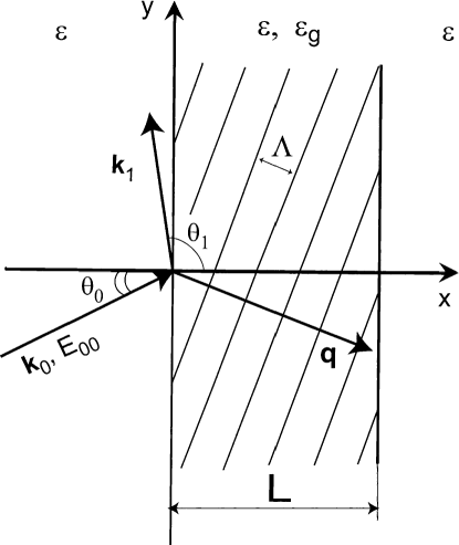
Figure 1: The scheme for grazing-angle scattering of bulk TE electromagnetic waves in a slanted holographic grating of width $L$ and grating amplitude $\epsilon_{g}$. The angle of incidence is $\theta_{0}$ and the amplitude of the incident wave in front of the grating is $E_{00}$. The Bragg condition is satisfied precisely for the first diffracted order (scattered wave) that propagates at an angle $\theta_{1}$ that is close to $\pi/2$ (i.e. at a grazing angle with respect to the grating boundaries).

Consider an isotropic medium with a volume, uniform, holographic grating represented by sinusoidal variations of the dielectric permittivity (Fig. 1):

$$\epsilon_{s} = \epsilon+\epsilon_{g}\exp(\mathrm{i}q_{x}x+\mathrm{i}q_{y}y)+\epsilon_{g}^{\ast}\exp(-\mathrm{i}q_{x}x-\mathrm{i}q_{y}y)$$

$$\textrm{if}\,\,\,\,0<x<L,$$

$$\epsilon_{s}=\epsilon\,\,\,\,\textrm{if}\,\,\,\,x<0\,\,\,\,\textrm{or}\,\,\,\,x>L,$$ (1)

where $L$ is the width and eg is the amplitude of the grating, the mean dielectric permittivity, $\epsilon$, is the same throughout the structure (see Eq. (1)), $q_{x}$ and $q_{y}$ are the $x$- and $y$-components of the reciprocal lattice vector $\mathbf{q}$, $q=2\pi/\Lambda$, $\Lambda$ is the period of the grating; the co-ordinate system is shown in Fig. 1. It is also assumed that there is no dissipation of electromagnetic waves inside and outside the grating ($\epsilon$ is real and positive), and the structure is infinite along the $y$- and $z$-axes. A bulk TE electromagnetic plane wave with the amplitude $E_{00}$ and wave vector $\mathrm{k}_{0}$ is incident onto the grating at an angle $\theta_{0}$ in the $xy$-plane—Fig. 1 (non-conical scattering).

The solutions inside and outside the non-uniform grating can be written as [9–11]:

$$E_{1}(x,y)=\sum_{n=-\infty}^{+\infty}S_{n}(x)\exp(\mathrm{i}k_{nx}x+\mathrm{i}k_{ny}y),$$ (2)

$$E|_{x<0}=E_{00}\exp(\mathrm{i}\mathbf{k}_{0}\cdot\mathbf{r})+\sum_{n=-\infty}^{+\infty}A_{n}\exp(\mathrm{i}\mathbf{k}_{\mathrm{r}n}\cdot\mathbf{r}),$$ (3)

$$E|_{x>L}=\sum_{n=-\infty}^{+\infty}B_{n}\exp(\mathrm{i}\mathbf{k}_{\mathrm{t}n}\cdot\mathbf{r}-\mathrm{i}k_{\mathrm{t}nx}L),$$ (4)

where the dependence of the field on time, i.e. the factor $\exp(-\mathrm{i}\omega t)$, is omitted, $k_{nx}$ and $k_{ny}$ are the $x$- and $y$-components of the wave vectors $\mathbf{k}_{n}$ determined by the Floquet condition:

$$\mathbf{k}_{n}=\mathbf{k}_{0}-n\mathbf{q}\,\,\,\,(n=0,\pm 1,\pm 2,...)$$ (5)

and the components of the wave vectors $\mathbf{k}_{\mathrm{r}n}$ and $\mathbf{k}_{\mathrm{t}n}$ of the nth reflected and transmitted waves in the regions $x<0$ and $x>L$ are determined by the equations:

$$k_{\mathrm{r}ny}=k_{\mathrm{t}ny},\,\,\,\,k_{\mathrm{r}nx}=-k_{\mathrm{t}nx}=-(k_{0}^{2}-k_{ny}^{2})^{1/2}.$$ (6)

If $k_{ny}\leq k_{0}$, then $k_{\mathrm{r}nx}\leq 0$ and $k_{\mathrm{t}nx}\geq 0$ (propagating waves), while if $k_{ny}>k_{0}$, then Im$(k_{\mathrm{r}nx})<0$ and Im$(k_{\mathrm{t}nx})>0$ (evanescent waves).

The Bragg condition is assumed to be satisfied precisely for the $+1$ diffracted order in Eq. (2) for all angles of scattering h1 that are assumed to be close to $\pi/2$ (the geometry of GAS—Fig. 1). The fact that the Bragg condition is satisfied precisely for all values of $\theta_{1}$ means that we have to adjust the grating parameters (the period and slanting angle) for each value of $\theta_{1}$. This is inconvenient in practice, but allows the analysis of GAS at optimal conditions, i.e. separately from the effects of small detunings of the Bragg condition (the same was done in [1] for the approximate theory of GAS).

The $x$-dependencies of amplitudes of the diffracted orders inside the grating are obtained from the solution of the truncated rigorous coupled wave equations and the boundary conditions at the grating boundaries $x=0,L$. As mentioned above, the rigorous analysis of the coupled wave equations and boundary conditions is carried out by means of the numerically stable enhanced T-matrix algorithm developed by Moharam et al. [10,11].

3 GAS in gratings with small amplitude

As indicated in the introduction and paper [1], GAS is characterised by a strong resonance with respect to angle of scattering $\theta_{1}$ (GAS resonance) only if the grating width $L$ is greater than the critical width $L_{c}$. Therefore, in this paper, we will consider mainly wide gratings with $L>L_{c}$. Physically, half of the critical width is equal to the distance within which the scattered wave can be spread across the grating by means of the diffractional divergence, before being re-scattered by the grating [7,8]. Two simple methods for the determination of Lc have been described in [7,8].

For example, consider a volume holographic grating with the parameters: $\epsilon=5$, $\theta_{0}=\pi/4$, and the wavelength in vacuum $\lambda=1\mu$m. The grating amplitude eg and grating width will be varied below (however, we will always have $L>L_{c}$). The Bragg condition is assumed to be satisfied precisely for the $+1$ diffracted order, i.e. in Eq. (5), $k_{1}=\epsilon^{1/2}\omega c$, and $\mathbf{k}_{1}$ is almost parallel to the grating boundaries—Fig. 1.

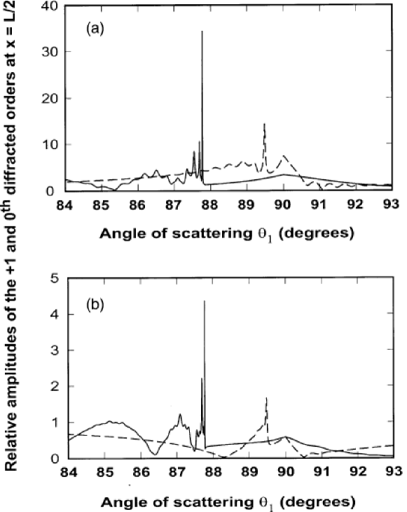
Figure 2: The rigorous dependencies of the relative amplitudes of (a) the scattered wave (the $+1$ diffracted order), $|S_{1}/E_{00}|$, and (b) the incident wave (the 0th diffracted order), $|S_{0}/E_{00}|$, in the middle of the grating (i.e. at $x=L/2$) on angle of scattering $\theta_{1}$. The structural parameters: $\epsilon=5$, $\theta_{0}=45^{\circ}$, the wavelength $\lambda(\mathrm{vacuum})=1\mu$m, $L=64.5\mu$m, the period and orientation of the gratings are determined by the Bragg condition and $\theta_{1}$. Dashed curves: $\epsilon_{g}=5\times 10^{-3}$; solid curves: $\epsilon_{g}=5\times 10^{-2}$.

Typical rigorous dependencies of amplitudes of the $+1$ and 0th diffracted orders (the scattered and incident waves) in the middle of the grating (i.e. at $x=L/2$) on angle of scattering h1 are presented in Figs. 2(a) and (b) for the gratings of width $L=64.5\mu$m, and $\epsilon_{g}=5\times 10^{-3}$ (dashed curves) and $\epsilon_{g}=5\times 10^{-2}$ (solid curves). The reasons for choosing $L=64.5\mu$ will become clear below.

It can be seen that a very strong resonant increase of the scattered (Fig. 2(a)) and incident (Fig. 2(b)) wave amplitudes occurs at a resonant angle of scattering $\theta_{1\mathrm{r}}<\pi/2$, i.e. when the scattered wave propagates at a grazing angle into the grating. It is important that these amplitudes in the GAS resonance are much larger than those typical for EAS (i.e. at $\theta_{1}=\pi/2$—Figs. 2(a) and (b)). It can also be seen that the larger the grating amplitude, the stronger the GAS resonance—compare solid and dashed curves in Figs. 2(a) and (b) (the same conclusion as in the approximate theory [1]). In addition, the resonant angle noticeably decreases with increasing grating amplitude (Figs. 2(a) and (b)).

Similarly to the approximate theory, the rigorous analysis suggests that the GAS resonance increases with increasing grating width $L$. It can also be seen that for given structural parameters there is a set of approximately periodically spaced optimal grating widths $L_{\mathrm{opt}}$ for which the scattered wave amplitude outside the grating is zero (amplitudes $A_{1}$ and $B_{1}$ in Eqs. (3) and (4) are zero), and the energy of the scattered wave is entirely concentrated within the grating region—see also [1]. Recall that since the mean dielectric permittivity is the same inside and outside the grating (see Eq. (1)), there is no conventional guiding effect in the grating. The entire localisation of the scattered wave inside the grating (at $L=L_{\mathrm{opt}}$) is achieved due to peculiarities of scattering, re-scattering and diffractional divergence (similarly to the approximate theory [1]). It can also be seen that the values of Lopt and the corresponding resonant angles of scattering $(\theta_{1\mathrm{r}})_{\mathrm{opt}}$ obtained from the rigorous theory at $\epsilon_{g}=5\times 10^{-3}$ (small grating amplitude) are only insignificantly different from those obtained in the approximate theory [1], if the grating width does not exceed $\approx 100\mu$m. At the same time, for very large grating widths, or large grating amplitudes, the rigorous theory gives different values of $L_{\mathrm{opt}}$. These values can be found in the rigorous theory in the same way as it was done in [1]. The considered grating width $L=64.5\mu$m (Figs. 2(a) and (b)) is one of $L_{\mathrm{opt}}$ if $\epsilon_{g}=5\times 10^{-3}$ (dashed curves in Figs. 2(a) and (b)).

However, it is important to remember that strong GAS resonance occurs not only at $L=L_{\mathrm{opt}}$, but at any other width that is larger than the critical width (for the considered structures, $L_{c}\approx 28\mu$m for $\epsilon_{g}=5\times 10^{-3}$, and $L_{c}\approx 6.5\mu$m for $\epsilon_{g}=5\times 10^{-2}$ [7,8])—see solid curves in Figs. 2(a) and (b). The main effect of optimal grating widths for small grating amplitudes is the total localisation of the scattered wave inside the grating. If the grating amplitude is larger than $\approx 0.1\epsilon$, then at $L=L_{\mathrm{opt}}$, the scattered wave amplitude at the grating boundaries may be of the order of the incident wave amplitude in front of the grating (see below).

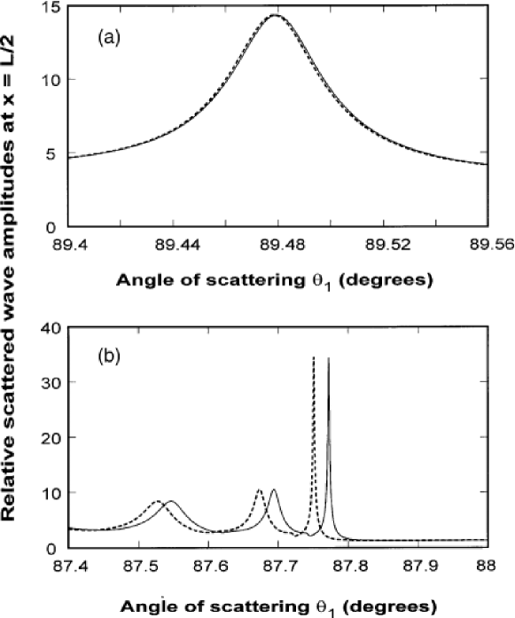
Figure 3: The comparison of the rigorous angular dependencies of the scattered wave amplitudes in the middle of the grating, presented in Fig. 2(a) (solid curves), with the same dependencies obtained from the approximate theory [1] (dotted curves). (a) $\epsilon_{g}=5\times 10^{-3}$, (b) $\epsilon_{g}=5\times 10^{-2}$.

If we plot the corresponding approximate curves (obtained in [1]) in Figs. 2(a) and (b), we will hardly notice any difference from the presented rigorous curves. However, this is not because the approximate and rigorous theories give the same results, but rather the scale in Figs. 2(a) and (b) is too small to see the differences between the curves near sharp resonances. Therefore, Figs. 3(a) and (b) present the rigorous and approximate angular dependencies of the scattered wave amplitudes just near the GAS resonance. It can clearly be seen that if the GAS resonance is not very strong and the grating amplitude is small, then the agreement between the approximate and rigorous theories is very good (within $\approx 2$%—Fig. 3(a)). At the same time, if the grating amplitude is increased 10 times, then the GAS resonance becomes much stronger and sharper, which results in significant discrepancies between the approximate and rigorous theories (Fig. 3(b)). Note however that these discrepancies are mainly limited to variations of the resonant angle of scattering. Indeed, as seen from Figs. 3(a) and (b), the shape and the height of maximums of the rigorous and approximate dependencies are practically identical, and the only difference is that the rigorous curve is slightly shifted to the right (in the direction of larger angles of scattering). That is, values of the resonant angle $\theta_{1\mathrm{r}}$ in the rigorous theory are larger than those predicted by the approximate theory [1].

It is interesting that reducing the angle of incidence $\theta_{0}$ results in noticeably better agreement between the approximate and rigorous theories, despite increasing strength of the GAS resonance for smaller angles of incidence. For example, if the angle of incidence $\theta_{0}=0$, then the maximums similar to those in Fig. 3(b) practically merge, and the corresponding discrepancies between the approximate and rigorous theories are no more than those in Fig. 3(a).

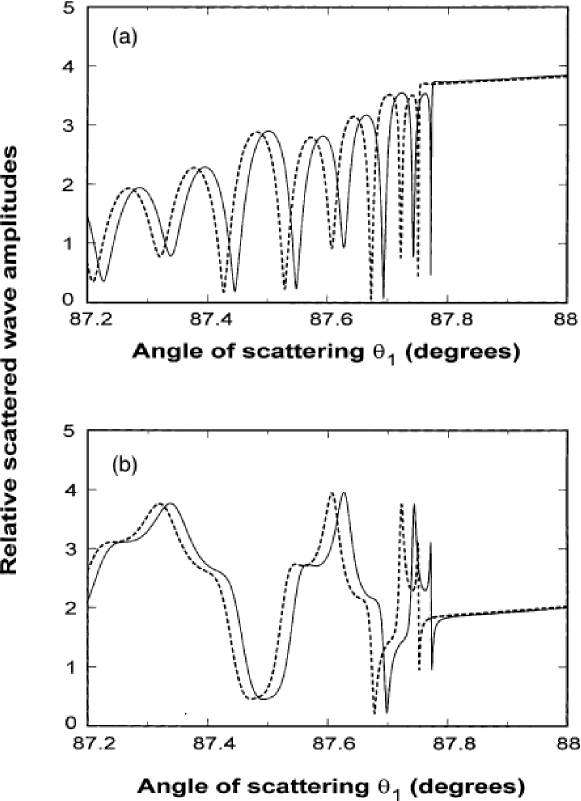
Figure 4: The comparison of the rigorous (solid curves) and approximate (dotted curves) angular dependencies of the scattered wave amplitudes at the front (a) and rear (b) grating boundaries for the structure corresponding to the solid curves in Figs. 2(a) and (b) (and to Fig. 3(b)), i.e. with $\epsilon_{g}=5\times 10^{-2}$, $\epsilon=5$, $\theta_{0}=45^{\circ}$, $\lambda(\mathrm{vacuum})=1\mu$m, $L=64.5\mu$m.

Similar conclusions can be drawn when considering rigorous angular dependencies of the scattered wave amplitudes at the front and rear boundaries of the grating with $\epsilon_{g}=5\times 10^{-2}$—Figs. 4(a) and (b). These dependencies are practically the same as those obtained by means of the approximate theory [1], except for that they are slightly shifted towards larger angles of scattering by the same value as the rigorous curves in Fig. 3(b). Decreasing angle of scattering results in better agreement between the approximate and rigorous theories.

Note that this result is fairly unexpected. One could think that taking into account higher diffracted orders in the rigorous theory should result in significant changes in the pattern of scattering, especially in the case of strong and sharp oscillations as in Fig. 4. In particular, these expectations could be related to additional energy losses from the grating due to boundary scattering and additional propagating orders outside the grating [9]. However, as seen from Figs. 2–4, the only effect of higher diffracted orders in the rigorous theory is a slight shift of the corresponding dependencies towards larger angles of scattering. In particular, this is probably because GAS is characterised by a strong resonant increase of the incident and scattered wave amplitudes in the middle of the grating, while at the boundaries ($x=0$ and $x=L$) the scattered wave amplitudes normally do not exceed a few amplitudes of the incident wave, especially if the grating amplitude is large. Moreover, if $L=L_{\mathrm{opt}}$ and $\theta_{1}=(\theta_{1\mathrm{r}})_{\mathrm{opt}}$, then the scattered wave amplitude at the grating boundaries and outside the grating is approximately zero. Therefore, the amplitudes of propagating orders outside the grating (in particular, the amplitude of boundary scattered wave) must be small, as well as the associated energy losses. Thus their effect on the pattern of scattering is limited.

4 Scattering in gratings with large amplitude

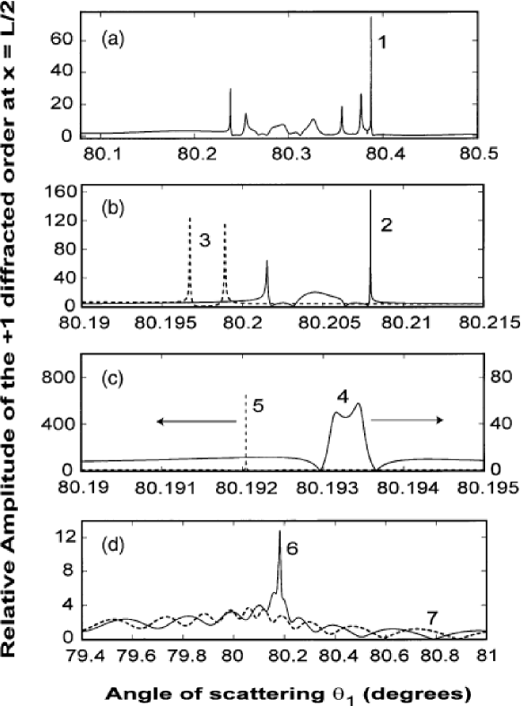
Figure 5: The rigorous dependencies of the relative scattered wave amplitude $|S_{1}/E_{00}|$ in the middle of the grating on angle of scattering $\theta_{1}$ for large grating amplitudes: (1) $\epsilon_{g}=0.55$, (2) $\epsilon_{g}=0.59$, (3) $\epsilon_{g}=0.593$, (4) $\epsilon_{g}=0.595$, (5) $\epsilon_{g}=\epsilon_{gc1}\approx 0.595562$, (6) $\epsilon_{g}=0.6$, (7) $\epsilon_{g}=0.65$. The other structural parameters are as for Figs. 2–4.

All the results and tendencies presented in the previous section are true not only for very small grating amplitudes (Figs. 2–4), but also for values of $\epsilon_{g}$ up to $\approx 10$% of the mean dielectric permittivity in the grating (for the considered gratings this is $\epsilon_{g}\approx 0.5$). However, when the grating amplitude approaches $approx0.1\epsilon$, the rigorous pattern of GAS changes substantially. For example, if the grating amplitude $\epsilon_{g}=0.55$ and all other parameters are the same as for Figs. 2–4, then the rigorous dependencies of the scattered (and incident) wave amplitude on angle of scattering $\theta_{1}$ in the middle of the grating display sharp oscillations between two distinct resonant peaks (Fig. 5(a)). Outside the range of angles between these two peaks the scattered wave amplitude is relatively small and only weakly depends on $\theta_{1}$—Fig. 5(a). Increasing grating amplitude results in shifting these two peaks towards each other—see Fig. 5(b). In this case both the peaks become rapidly sharper and higher. This is especially relevant to the left maximum that may even overtake the main GAS resonance (i.e. the right maximum in Fig. 5(a) and (b)). The number of peaks in between the extreme left maximum and the extreme right maximum reduces with increasing grating amplitude. Finally, the two extreme maximums come so close to each other that they can hardly be resolved (solid curve in Fig. 5(c)) and then merge together in one extremely sharp and high maximum (dotted curve in Fig. 5(c)). The merger occurs at a critical grating width $\epsilon_{gc1}$ (the reason for using the index 1 in $\epsilon_{gc1}$ will be clear below). In the considered case, $\epsilon_{gc1}=0.595562$—Fig. 5(c). Further increase of the grating amplitude results in a rapid decrease of the GAS resonance at $\epsilon_{g}=0.6$—solid curve in Fig. 5(d), with its complete disappearance at $\epsilon_{g}=0.65$—-dotted curve in Fig. 5(d).

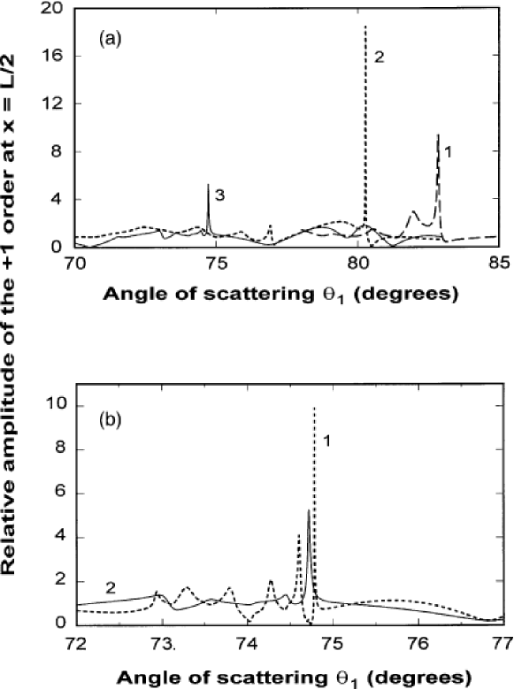
Figure 6: The same dependencies as in Fig. 5, but for different grating width $L=20\mu$m, and the following grating amplitudes: (1) $\epsilon_{g}=0.38$, (2) $\epsilon_{g}=0.44$, (3) $\epsilon_{g}=0.51$, (4) $\epsilon_{g}=0.565$, (5) $\epsilon_{g}=0.58$, (6) $\epsilon_{g}=0.5868$.

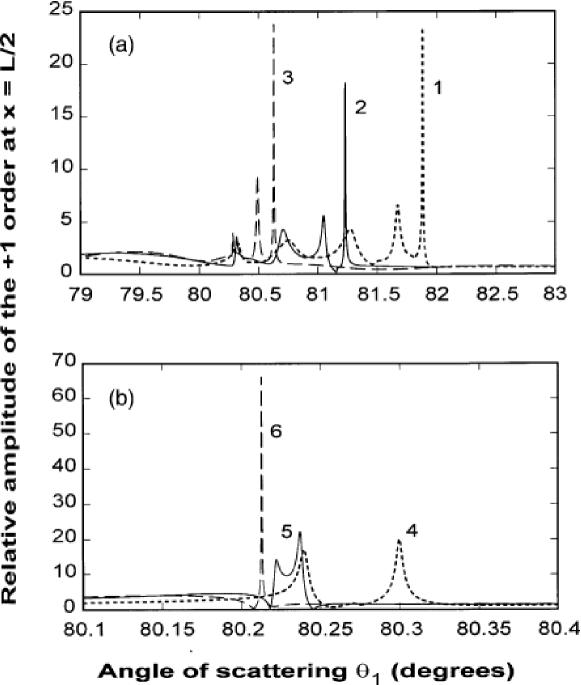
Figure 7: (a) The rigorous dependencies of the relative scattered wave amplitude $|S_{1}/E_{00}|$ in the middle of the grating on angle of scattering $\theta_{1}$ for the grating with $L=10\mu$m and (1) $\epsilon_{g}=0.3$, (2) $\epsilon_{g}=\epsilon_{gc1}\approx 0.567$, (3) $\epsilon_{g}=0.8$. (b) The second GAS resonance. The comparison of the rigorous dependencies of the relative scattered wave amplitudes in the middle of two gratings of different widths: (1) $L=20\mu$m, $\epsilon_{g}=0.8$, (2) $L=10\mu$m, $\epsilon_{g}=0.8$ (i.e. curve 2 is the same as curve 3 in (a)). The other structural parameters are as before: $\epsilon=5$, $\theta_{0}=45^{\circ}$, $\lambda(\mathrm{vacuum})=1\mu$m.

The presence of a critical grating amplitude $\epsilon_{gc1}$, at which the two extreme maximums merge, producing an extremely strong resonance (with its subsequent rapid reduction for $\epsilon_{g}>\epsilon_{gc1}$, is the general feature of GAS in different gratings. In particular, it can be seen that generally $\epsilon_{gc1}$ depends on grating width. However, this dependence is weak. For example, for gratings of $L=64.5\mu$m (Fig. 5), $L=20\mu$m (Fig. 6), and $L=10\mu$m (Fig. 7a) the values of the critical grating amplitude are 0.595562, 0.5868, and 0.567, respectively. The main features of the pattern of GAS in gratings of smaller widths are the same as for the grating with $L=64.5\mu$m (compare Figs. 5–7(a)). However, the typical height and sharpness of the resonance maximums are significantly reduced when the grating width is reduced—Figs. 6 and 7(a). This is similar to the general tendency for GAS obtained by means of the approximate theory [1]. At the same time, it is important to understand that the approximate theory completely fails to predict the actual pattern of GAS at large grating amplitudes, in particular, in the vicinity of the critical grating amplitude.

Note that increase of height of the resonance is not monotonous with increasing grating amplitude—see curves 1–3 in Fig. 6(a). This is partly because the grating width $L=20\mu$m is approximately equal to one of the optimal widths $L_{\mathrm{opt}}$ for the grating amplitudes $\epsilon_{g}=0.38,0.51,0.5868$.

Curves 2 and 3 in Fig. 7(a) also indicate another highly unusual and unexpected feature of scattering, that can be revealed only using the rigorous theory. Indeed, when the two limiting maximums discussed above merge together (at $\epsilon_{g}=\epsilon_{gc1}$) and result in a very strong and sharp resonance (dotted curve in Fig. 5c, and curves 3 and 2 in Figs. 6(b) and 7(a), respectively), there appears another peak at a significantly smaller angle of scattering—see the small sharp bump on curve 2 in Fig. 7(a) at about $77^{\circ}$. When the grating amplitude is increased ($\epsilon_{g}>\epsilon_{gc1}$), this maximum increases substantially and turns into a strong resonance—curve 3 in Fig. 7(a). Note that this is not the same maximum corresponding to the described GAS resonance, shifted towards smaller angles. Indeed, it appears when the GAS resonance is still strong (curve 2 in Fig. 7(a)). We will call this maximum second GAS resonance. It exists not only in the considered grating of $L=10\mu$m. For example, Fig. 7(b) presents the comparison of the second GAS resonance for two gratings of $L=20\mu$m (curve 1) and $L=10\mu$m (curve 2, which the same as curve 3 in Fig. 7(a)). In particular, Fig. 7(b) demonstrates the general tendency that, similar to the first GAS resonance, the second GAS resonance becomes stronger and sharper with increasing grating width (compare the main maximums for curves 1 and 2 in Fig. 7(b)). However, it is interesting that the angle of scattering, at which the second GAS resonance occurs, is almost independent of grating width (Fig. 7(b)). This is again similar to the first GAS resonance—compare for example dotted curve in Fig. 5c with curves 3 and 2 in Figs. 6(b) and 7(a), respectively.

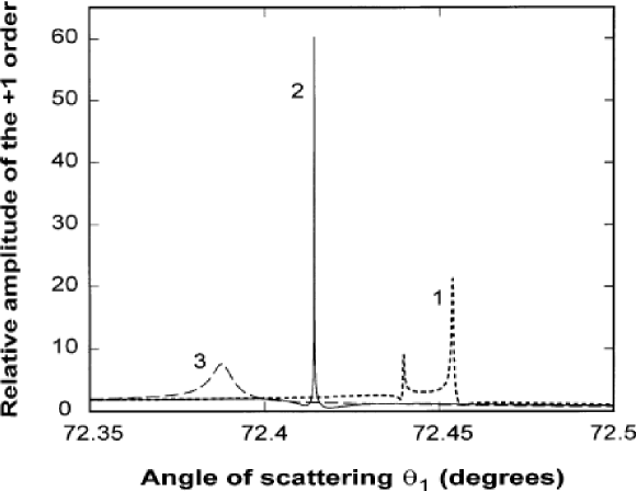
Figure 8: The second GAS resonance in the grating of $L=20\mu$m, $\epsilon=5$, $\theta_{0}=45^{\circ}$, $\lambda(\mathrm{vacuum})=1\mu$m, and (1) $\epsilon_{g}=1.12$, (2) $\epsilon_{g}=\epsilon_{gc2}\approx 1.1309$, (3) $\epsilon_{g}=1.14$.

In addition, the whole pattern of scattering near the second GAS resonance is very similar to that demonstrated by Figs. 5(a)–(c) and 6(a) and (b) near the first GAS resonance. For example, on the right of the main resonant maximum the angular dependence of the scattered wave amplitude in the middle of the grating is fairly smooth, whereas on the left it is characterised by a number of oscillations with sharp maximums (Fig. 7(b)). The larger the grating width, the larger the typical amplitude and number of these oscillations (compare curves 1 and 2 in Fig. 7(b)). If the grating amplitude is increased, these oscillations appear to be confined to an angular interval between two distinct maximums in exactly the same fashion as it was for the first GAS resonance—see Figs. 5(a) and (b) and 6(a). One of these limiting maximums is the main maximum corresponding to the second GAS resonance in Fig. 7(b), and the other one is just appearing at the angle of about $73^{\circ}$. Further increase of the grating amplitude results in a significant increase of both these limiting maximums. In the same way as for the first GAS resonance (Figs. 5 and 6), increasing grating amplitude results in shifting the limiting maximums (in the second GAS resonance) towards each other with the simultaneous reduction of the number of oscillations between them (compare curves 1 in Figs. 8 and 7(b) with curves in Figs. 6(a) and (b)). Finally, when the grating amplitude reaches the second critical value $\epsilon_{g}=\epsilon_{gc2}$ (the index 2 stands for the second GAS resonance), the two limiting maxi- mums merge together producing a very strong and sharp resonance—curve 2 in Fig. 8. Further increase of the grating amplitude results in a rapid decrease of the second GAS resonance (curve 3 in Fig. 8), which is very similar to the first GAS resonance—Fig. 5(d).

Note also that the height of the second GAS resonance at $\epsilon_{g}=\epsilon_{gc2}$ is very close to that of the first GAS resonance at $\epsilon_{g}=\epsilon_{gc1}$—compare curves 2 and 3 in Figs. 8 and 6(b), respectively. This statement is more accurate for gratings of larger width. It is also interesting that the value of $\epsilon_{gc2}$ is approximately 2 times larger than $\epsilon_{gc1}$.

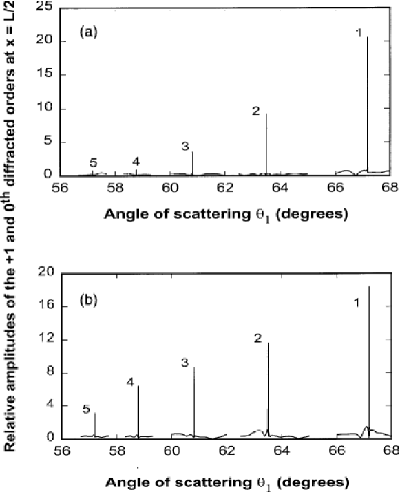
Figure 9: The rigorous dependencies of amplitudes of the scattered (a) and incident (b) waves in the middle of the grating (i.e. at $x=L/2$) at the critical grating amplitudes $\epsilon_{gci}$ ($i=3,4,5,6,7$) for the $i$th GAS resonance: (1) $\epsilon_{g}=\epsilon_{gc3}\approx 1.50988$, (2) $\epsilon_{g}=\epsilon_{gc4}\approx 1.763$, (3) $\epsilon_{g}=\epsilon_{gc5}\approx 1.9357$, (4) $\epsilon_{g}=\epsilon_{gc6}\approx 2.055$, (5) $\epsilon_{g}=\epsilon_{gc7}\approx 2.1407$. The other structural parameters: $L=20\mu$m, $\epsilon=5$, $\theta_{0}=45^{\circ}$, $\lambda(\mathrm{vacuum})=1\mu$m.

Very strong similarities between the patterns of scattering in the first and the second GAS resonances suggest that when the second GAS resonance disappears at $\epsilon_{g}>\epsilon_{gc2}$, it is reasonable to expect another resonance (third GAS resonance) to appear at smaller angles of scattering and larger grating amplitudes. This is indeed the case, and this third GAS resonance is characterised by the same pattern of scattering. That is, when the second GAS resonance is suppressed by increasing $\epsilon_{g}$ above $\epsilon_{gc2}$, there appear two distinct maximums at angles that are several degrees less than the angle at which the second GAS resonance occurs at $\epsilon_{g}=\epsilon_{gc2}$. These maximums increase with increasing grating amplitude and shift towards each other. Oscillations of the angular dependence of the scattered wave amplitude occur only between these two limiting maximums (in exactly the same way as it was for the first and the second GAS resonances—Figs. 5(a) and (b), 6(a), and 7(b)). Finally, these limiting maximums merge together, producing a very strong and sharp resonance, and this occurs at $\epsilon_{g}=\epsilon_{gc3}$. Further increase of $\epsilon_{g}$ results in a rapid decrease of the third GAS resonance. After that, the fourth GAS resonance appears at larger grating amplitude and a smaller angle of scattering, and so on. The corresponding resonant dependencies of the scattered wave amplitudes in the middle of the grating of $L=20\mu$m and $\epsilon_{g}=\epsilon_{gci}$, where $i=3,4,5,6,7$, are presented in Fig. 9(a).

Fig. 9(a) clearly demonstrates that unlike the second GAS resonance at $\epsilon_{g}=\epsilon_{gc2}$, that is almost the same in height as the first GAS resonance at $\epsilon_{g}=\epsilon_{gc1}$, the third, fourth, etc. resonances at $\epsilon_{g}=\epsilon_{gci}$ are significantly smaller. For example, the height of the seventh GAS resonance in the grating of $L=20\mu$m is only $\approx 0.76E_{00}$, where $E_{00}$ is the amplitude of the incident wave at the front boundary—curve 5 in Fig. 9(a). Note also that height of all the GAS resonances strongly depends on grating width (unlike the values of angles and grating amplitudes at which these resonances occur). For example, the height of the first two GAS resonances at $\epsilon_{g}=\epsilon_{gc1,2}$ is $\approx 670E_{00}$ for $L=64.5\mu$m, while for $L=20\mu$m they are $\approx 10$ times smaller (Figs. 6(b) and 8). Similarly, the seventh GAS resonance at $L=20\mu$m (curve 5 in Fig. 9(a)) is also $\approx 10$ times smaller in height than the same seventh resonance at $L=64.5\mu$m. It is interesting that resonance half-width is practically the same for all the maximums in Fig. 9(a), despite the significant decrease in their height with increasing grating amplitude (all these maximums, including those of curves 3 and 2 in Figs. 6(a) and 8, have the half-widths $\approx 3\times 10^{-4}$ deg). At the same time, the half-width of the resonances noticeably increases (decreases) with decreasing (increasing) grating width. For example, the half-width of the maximum of curve 2 in Fig. 7(a) is $\approx 0.01^{\circ}$.

Decreasing angle of incidence results in a noticeable increase of the height and sharpness of the predicted resonances. In addition, the resonant angles of scattering decrease, and the critical grating amplitude, at which the merger of two limiting maximums occurs, increases with decreasing angle of incidence. For example, if $L=64.5\mu$m and $\theta_{0}=20^{\circ}$ (compared to $\theta_{0}=45^{\circ}$ for Figs. 2–5), then $\epsilon_{gc1}=1.654118$, the corresponding resonant angle $\theta_{1}\approx 73.039^{\circ}$, and the height of the resonance $\approx 1300E_{00}$ (compare with $\epsilon_{gc1}=0.595562$, $\theta_{1}\approx 80.192^{\circ}$, and the resonance height $\approx 740E_{00}$ for the dotted curve in Fig. 5c).

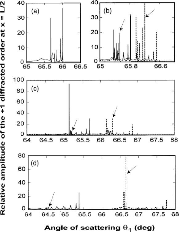
Figure 10: Small angles of incidence (near-normal incidence). The rigorous dependencies of the relative scattered wave amplitude in the middle of the grating of $L=10\mu$m, $\epsilon_{g}=4$, $\epsilon=5$, $\lambda(\mathrm{vacuum})=1\mu$m. (a) $\theta_{0}=0^{\circ}$, (b) $\theta_{0}=0.3^{\circ}$ (dotted curve), $\theta_{0}=-0.3^{\circ}$ (solid curve), (c) $\theta_{0}=0.5^{\circ}$ (dotted curve), $\theta_{0}=-0.5^{\circ}$ (solid curve), (d) $\theta_{0}=1^{\circ}$ (dotted curve), $\theta_{0}=-1^{\circ}$ (solid curve). The arrows indicate the middle maximum that splits from the right limiting maximum at $\theta_{0}\neq 0$ and shifts towards the left limiting maximum with increasing $|\theta_{0}|$.

If the angle of incidence is close to zero (almost normal incidence onto the grating), the pattern of scattering noticeably changes. This is illustrated by Fig. 10, presenting the dependencies of the amplitude of the scattered wave ($+1$ diffracted order) on angle of scattering in the middle of the grating of $L=10\mu$m. If $\theta_{0}=0^{\circ}$, then we obtain the pattern with two strong limiting maximums, similar to that in Figs. 5(a) and (b) and 6(a) (though appearing at much larger grating amplitudes: $\epsilon_{g}=4$ in Fig. 10(a)). However, if the angle of incidence is slightly different from 0, then the right limiting maximum in Fig. 10(a) splits into two, and there are three distinct maximums in the pattern. The middle (out of three) maximum is indicated by the arrows in Figs. 10(b)–(d). As $|\theta_{0}|$ increases from zero, this middle maximum splits off the right limiting maximum in Fig. 10(a) and shifts towards the left limiting maximum. Already when $\theta_{0}=\pm 0.3^{\circ}$ (Fig. 10(b)), the pattern of scattering is substantially different from what it was at $\theta_{0}=0^{\circ}$ (Fig. 10(a)). The middle maximum in Fig. 10(b) is already more than half way through from the right limiting maximum to the left. Note that for negative values of $\theta_{0}$ the middle maximum shifts closer to the left limiting maximum than for the same positive values (compare solid and dotted curves in Fig. 10(b)). If $|\theta_{0}|$ is increased further, the middle maximum may vary strongly in height and sharpness (Figs. 10(b–d)). Finally, the middle and the left maximums for $\theta_{0}<0$ (solid curves) merge together, producing a very high resonance, and further increase of $|\theta_{0}|$ quickly results in annihilation of both the maximums (solid curve in Fig. 10(d)). A similar pattern is observed when the angle $\theta_{0}$ in increased from zero—see the dotted curves in Figs. 10(b)–(d). However, in this case the merger of the left and the middle maximums occur at larger values of $\theta_{0}$—compare Figs. 10(c) and (d). The right limiting maximum tends to decrease with increasing $\theta_{0}$. Therefore, it may have noticeable height only at almost normal incidence—typically for $\theta_{0}\leq 5^{\circ}$.

From here, we can see the relationship between the pattern of scattering presented by Figs. 5–7a for large incidence angles and the pattern shown by Fig. 10. As mentioned above, decreasing (increasing) angle of incidence results in increasing (decreasing) values of $\epsilon_{gc1}$. Therefore, instead of fixing $\theta_{0}$ and finding $\epsilon_{gc1}$, we can fix $\epsilon_{g}$ and choose the critical angle of incidence $\theta_{0c}$ corresponding to the merger of the maximums. This suggests that the middle and the left limiting maximums in Figs. 10(b)–(d) correspond to the two limiting maximums considered in Figs. 5–7a. The right limiting maximum in Figs. 10(b)–(d) could not be seen in Figs. 5–7a since it is negligible at large angles of incidence.

Note also that according to the tendency mentioned above, resonant angles of scattering decrease with decreasing angle of incidence. This is also in obvious agreement with Figs. 10(a)–(d).

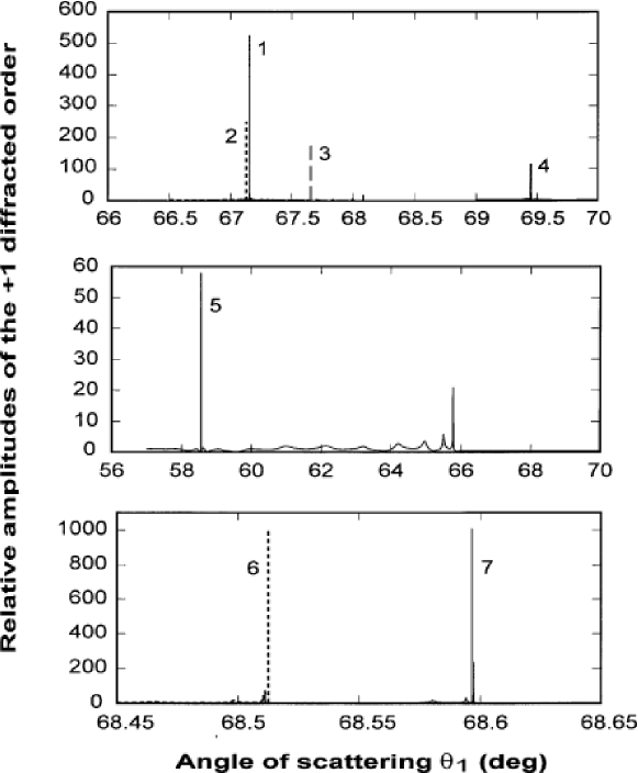
Figure 11: The rigorous dependencies of the scattered wave amplitude in the middle of the grating when the left and the middle maximums merge, i.e. at $\epsilon_{g}e=\epsilon_{gc1}$. The grating width is optimised for the strongest merged resonance in each grating. (1) $L=10\mu$m, $\epsilon_{g}e=\epsilon_{gc1}\approx 4.2439906$, $\theta_{0}=1^{\circ}$, resonance halfwidth $\delta\theta\approx 7\times 10^{-6}$ deg, (2) $L=9.93\mu$m, $\epsilon_{g}e=\epsilon_{gc1}\approx 3.53973$, $\theta_{0}=3^{\circ}$, $\delta\theta\approx 4\times 10^{-5}$ deg, (3) $L=10.05\mu$m, $\epsilon_{g}e=\epsilon_{gc1}\approx 3.1133$, $\theta_{0}=5^{\circ}$, $\delta\theta\approx 6\times 10^{-5}$ deg, (4) $L=9.97\mu$m, $\epsilon_{g}e=\epsilon_{gc1}\approx 2.4325$, $\theta_{0}=10^{\circ}$, $\delta\theta\approx 1.5\times 10^{-4}$ deg, (5) $L=10\mu$m, $\epsilon_{g}e=\epsilon_{gc1}\approx 2.3624$, $\theta_{0}=-3^{\circ}$, $\delta\theta\approx 4\times 10^{-5}$ deg, (6) $L=10.05\mu$m, $\epsilon_{g}e=\epsilon_{gc1}\approx 5.1491$, $\theta_{0}=0$, $\delta\theta\approx 9\times 10^{-7}$ deg, (7) $L=10\mu$m, $\epsilon_{g}e=\epsilon_{gc1}\approx 5.1823$, $\theta_{0}=0$, $\delta\theta\approx 3\times 10^{-7}$ deg.

As mentioned above, when the middle and the left limiting maximums in Figs. 10(b)–(d) merge, they produce extremely strong and sharp resonances (similar to those in Figs. 5c, 6b, 7a, 8 and 9). This merger can be achieved by choosing the right angle of incidence and/or grating amplitude. The resultant typical resonance maximums are presented in Fig. 11. The corresponding structural parameters and half-widths of the maximums are presented in the figure caption. Note that for all resonances in Figs. 11 the grating width has been optimised for maximal height of the main maximums. This is the reason for slight variations of the grating widths of the considered gratings.

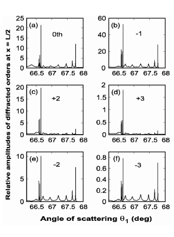
Figure 12: The rigorous dependencies of the relative amplitudes of the six diffracted orders (having significant amplitudes) on angle of scattering $\theta_{1}$ for the structure corresponding to the dotted curve in Fig. 10(d). The number of the particular diffracted order is indicated in each of the subplots.

It can be seen that decreasing angle of incidence results in a substantial increase of height of the merged maximums (compare curves 1–5 in Fig. 11). The smaller maximums of curves 5 and 3 (for curve 3 it occurs at $\approx 68.1^{\circ}$—Fig. 11(a)) correspond to the right limiting maximums in Figs. 10(b)–(d). For positive $\theta_{0}$, this maximum completely disappears at $\theta_{0}>10^{\circ}$, whereas for negative $\theta_{0}$ it is much more noticeable even for non-normal incidence (though still relatively small).

At normal incidence, there is no middle maximum (Fig. 10(a)), and the merger occurs between the two limiting maximums. The resultant merged resonance is especially strong—curve 6 in Fig. 11. In this case, further increase of the grating amplitude results in an oscillatory behaviour of the resonance. For example, increasing grating amplitude beyond the value corresponding to curve 6 ($\epsilon_{g}=5.1491$) results in a significant reduction of the resonance (to $\approx 300E_{00}$), and then in increasing it back to $\approx 1090E_{00}$ (at $\epsilon_{g}=5.1823$—see curve 7 in Fig. 11). Further increase of the grating amplitude results in other maximums that exceed several thousands of $E_{00}$.

It is obvious that the predicted extremely large amplitudes of the $+1$ diffracted orders, together with the large grating amplitude, must lead to very significant amplitudes of other diffracted orders in the Floquet expansion (2). This is demonstrated by Fig. 12, where amplitudes of several diffracted orders, other than the $+1$ order, are presented for the structure corresponding to the dotted curve in Fig. 10(d).

It can be seen that the amplitude of the incident wave (0th diffracted order) approximately follows the $+1$ diffracted order—compare the dotted curve in Fig. 10(d) and the curve in Fig. 12(a). This is similar to what has been predicted previously for GAS by means of the approximate and rigorous theories (see [1] and Fig. 2(b)). In particular, both the scattered and incident wave amplitudes experience a strong resonant increase in the middle of the grating. This is expected, since the extremely large scattered wave amplitude inside the grating must result in substantial re-scattering, as a result of which the incident wave must also have a large amplitude (note however that the energy conservation requires the incident wave amplitude at the rear grating boundary to be $\leq E_{00}$). The $+2$ diffracted order is also expected to be large, since it is directly coupled to the resonantly strong $+1$ diffracted order (Fig. 12c). However, what is really surprising is that the $-1$ diffracted order is significantly stronger than the 0th and $+2$ orders. This is unexpected, since the $-1$ order is not coupled directly to the resonantly strong scattered wave, and one could think that it should be weaker than the 0th and $+2$ orders. The rigorous analysis demonstrates that this expectation is not correct, and the amplitude of the $-1$ order is not only larger than those of the 0th and $+2$ orders, but is very close to the amplitude of the $+1$ order (i.e. scattered wave). The same situation is with the $-2$ order that has (in the middle maximum) the amplitude only $\approx 2$ times less than that of the $+2$ order, though it can be expected to be significantly smaller.

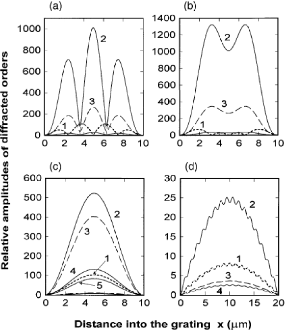
Figure 13: The rigorous $x$-dependencies of the relative amplitudes of several diffracted orders with noticeable amplitude inside the grating at the resonance angles of scattering $\theta_{1\mathrm{r}}$. The subplots (a)–(d) correspond to the resonances of curves 6, 7, 1 in Fig. 12, and curve 3 in Fig. 6, respectively. (a) 0th order (curve 1), $+1$ and $-1$ orders (curve 2), $+2$ and $-2$ orders (curve 3), $+3$ and $-3$ diffracted orders (lower solid curve); $\theta_{1}=\theta_{1\mathrm{r}}\approx 68.51250565^{\circ}$. (b) 0th order (curve 1), $+1$ and $-1$ orders (curve 2), $+2$ and $-2$ orders (curve 3), $+3$ and $-3$ diffracted orders (lower solid curve); $\theta_{1}=\theta_{1\mathrm{r}}\approx 68.59630026^{\circ}$. (c) 0th order (curve 1), $+1$ order (curve 2), $-1$ order (curve 3), $+2$ order (curve 4), $-2$ order (curve 5), $+3$ and $-3$ orders (lower dashed and solid curves, respectively); $\theta_{1}=\theta_{1\mathrm{r}}\approx 67.1545608^{\circ}$. (d) 0th order (curve 1), $+1$ order (curve 2), $-1$ order (curve 3), $+2$ order (curve 4); $\theta_{1}=\theta_{1\mathrm{r}}\approx 80.6295^{\circ}$.

This effect is even more obvious if we calculate amplitudes of the diffracted orders for the structures corresponding to curves 6 and 7 in Fig. 11. In this case, the angular dependencies of the amplitudes of the $-1$ and $+1$ orders are practically indistinguishable. The same is true for the $-2$ and $+2$ orders, $-3$ and $+3$ orders, etc. In addition, all these dependencies almost exactly reproduce the shape of curves 6 and 7 in Fig. 11 (though of different maximal heights). Therefore, presentation of these dependencies here is not worthwhile. Instead, Fig. 13 presents the typical $x$-dependencies of amplitudes of several diffracted orders in the gratings of widths $L\approx 10\mu$m (Fig. 13a–c) and $L=20\mu$m (Fig. 13(d)). The subplots in Fig. 13 correspond to the maximums of curve 6 in Fig. 11 (Fig. 13(a)), curve 7 in Fig. 11 (Fig. 13(b)), curve 1 in Fig. 11 (Fig. 13c), and curve 3 in Fig. 6(a) (Fig. 13(d)). In accordance with the mentioned above, the $x$-dependencies of the amplitudes of the $+1$ and $-1$ diffracted orders in Figs. 13(a) and (b) are practically indistinguishable and are both represented by curves 2. The match of these dependencies is better for Fig. 13(b), while in Fig. 13(a) there are minor differences near the two minimums of curve 2 in the grating (not shown in the figure). Similarly, each of curves 3 in Figs. 13(a) and (b) simultaneously represent the amplitudes of the $+2$ and $-2$ orders, and the lower solid curves in both the figures correspond to the $+3$ and $-3$ orders. This result is completely unexpected and surprising. Indeed, despite the obvious non-symmetry of the structure (Fig. 1) with respect to scattering into, for example, $+1$ and $-1$ orders (e.g., the Bragg condition is satisfied only for the $+1$ order), the amplitudes of these orders (and all other $+n$ and $-n$ orders) are practically indistinguishable in Figs. 13(a) and (b).

This however is not the case for less sharp and high resonances at larger angles of incidence—Figs. 13(c) and (d). In these figures, the amplitudes of the $+1$ and $-1$ orders (as well as those of the $+2$ and $-2$ orders, etc.) are noticeably different. Nevertheless, the stronger the resonance, the closer the amplitude of the $-1$ order to that of the $+1$ order (compare Figs. 13(c) and (d)). It is worth noting that strong resonances, as in Fig. 11, are highly sensitive to grating width. For example, if for curve 6 in Fig. 11 the grating width is changed from 10.02 to $10.1\mu$m, then the maximum of curve 6 in Fig. 11 reduces to $\approx 420E_{00}$ (i.e. more than two times compared to what it is in Fig. 11).

The small oscillations displayed by all the curves in Fig. 13(d) are also typical for other subplots in Fig. 13. However, due to much smaller scale, these oscillations are hardly seen on curves in Fig. 13a–c.

It is also important to realise that the presented results are not only relevant to the particular structural parameters considered above. It can be shown that the scaling procedure described in [12] is readily applicable to the considered gratings. For example, if the mean permittivity together with the grating amplitude are increased $\alpha$ times, then decreasing grating width $\alpha^{1/2}$ times must result in exactly the same results as for the gratings discussed above.

5 Eigenmodes of a slanted grating

The results obtained in Sections 3 and 4 demonstrate an extremely complex pattern of scattering, involving a number of strong resonances associated with strong increase of amplitudes of several diffracted orders inside the grating. It is obvious that a comprehensive physical explanation of all the predicted effects and resonant behaviour is hardly feasible at this stage. However, it is rather clear that diffractional divergence of the scattered wave, that has been used for the explanation of wave effects in the geometry of EAS [3–8], can hardly be used for the explanation of the predicted resonances. This is because if the grating amplitude is large, these resonances occur at angles of scattering significantly different from $\pi/2$. For example, at almost normal incidence, strong resonances have been found at angles of scattering $\theta_{1}$ between $40^{\circ}$ and $50^{\circ}$. It is hardly possible to expect that diffractional divergence of the $+1$ order (or any other diffraction order) can play a significant role at such angles of propagation with respect to the grating boundaries (see also [3–8]). Moreover, though the resonances were frequently referred to as GAS resonances in Section 4, one should not be deceived by this terminology, since in some cases the scattered wave no longer propagates at a grazing angle with respect to the grating boundaries (see also Figs. 9–12).

The explanation of the observed extremely strong resonances can be understood from Fig. 13. This figure demonstrates that in the strongest resonances, the amplitudes of the diffracted orders are resonantly large only inside the grating, whereas at its boundaries they are close to zero. On the other hand, any sufficiently strong resonance is associated with generation of some kind of eigen oscillations or eigenmodes in the structure. Therefore, the discovered resonances must be related to the resonant generation of a special new type of grating eigenmodes by an incident wave (the grating eigenmodes are coupled to the incident wave). Actually, these modes are not true structural eigenmodes, since if they were, they would have not been coupled to a incident wave. Due to the presence of this weak coupling, grating eigenmodes weakly leak from the grating. However, since the predicted resonances are extremely high (up to hundreds or even thousands of the amplitude of the incident wave), the leakage must be weak. In the case of a high resonance, the field in the grating represents, to a high degree of accuracy, the field in the corresponding grating eigenmode. Thus the field distribution presented in Fig. 13 is actually the field distribution in the grating eigenmodes. This is because the perturbation effect of the relatively weak incident wave (with $E_{00}\ll S_{1}|_{x=L/2}$) on the field distribution inside the grating is negligible.

It is important to recall that the considered gratings are not associated with any conventional guiding effect, since the mean dielectric permittivity $\epsilon$ is assumed to be the same inside and outside the grating (see Section 2 and Fig. 1). The guiding effect on the eigenmodes is imposed only by the grating. As a result, a grating of $10\mu$m width can guide a wave with the amplitude in the middle of the grating, that is thousands of times larger than at the grating boundaries. It is also interesting that all the gratings considered in this paper are oblique (slanted) gratings, which makes them asymmetric from the view-point of a mode propagating along the grating. Nevertheless, the field distribution in the modes corresponding to strong resonances is always practically symmetric with respect to the middle of the grating (Figs. 13(a)–(c)).

The discovered eigenmodes are formed by the interacting diffracted orders in the grating. This interaction occurs so that amplitudes of the diffracted orders decrease to about zero as they propagate towards a grating boundary. For example, the diffracted orders whose wave vectors point towards the rear grating boundary increase in amplitude (gaining energy from the diffracted orders “travelling” in the opposite direction) in the first half of the grating (from $x=0$ to $x=L/2$), and then lose their energy due to the same interaction in the second half of the grating. The opposite occurs for diffraction orders with the wave vectors pointing towards the front boundary.

Since we can consider a wave incident on the grating from its either side, the discovered eigenmodes can equally propagate in both directions along the grating, i.e. in the positive and negative directions of the $y$-axis in Fig. 1.

As can be seen from Fig. 13, the structure of the grating eigenmodes can be quite different, de- pending on structural parameters and angles of propagation of diffraction orders (i.e. mode type). These modes are significantly more complex than the conventional modes of a slab waveguide. This has also been demonstrated by the consideration of grating eigenmodes in the presence of the conventional guiding effect, i.e. in a guiding slab with a modulated dielectric permittivity [13]. In this case, a number of new grating eigenmodes are predicted, that are strongly different from the conventional guided modes in a slab (e.g., grating eigenmodes in a slab cannot exist in the absence of the grating) [13].

Note that without the consideration of the grating eigenmodes the discussed strong resonances, like those in Figs. 11(a)–(c), are practically useless. This is because they are very difficult to achieve in practice due to extremely large relaxation times, and thus impractically large apertures of the incident bean that would be required for the steady-state to be achieved. However, the existence of the grating eigenmodes radically changes the situation. The resonances are used only for the determination of the field structure of these modes that can be generated by other means, similar to those used for generation of the conventional slab modes.

Note also that especially strong resonances (and the described grating eigenmodes) are often obtained for very large grating amplitudes (e.g., $\epsilon_{g}\approx 3$ to 5). Recalling that, according to Eq. (1), the actual amplitude of modulation of the mean permittivity in the grating is equal to $2\mathrm{Re}(\epsilon_{g})$, we can see that $\epsilon_{g}\approx 5$ corresponds to the modulation amplitude $2\epsilon_{g}\approx 10$. This is 2 times larger than the mean permittivity in the structure. This means that the permittivity in the grating must vary from positive to negative values. On the other hand, negative permittivity can be obtained in metals, ionic crystals (between the frequencies of transverse and longitudinal optical phonons), or near any sufficiently strong material resonance. In this case, dissipation in the medium is inevitable. The accurate analysis of the grating eigenmodes and the associated resonances in the presence of dissipation is beyond the scope of this paper. However, it can be noted that small dissipation could, for example, be compensated by appropriate gain in the material of the grating.

6 Conclusions

In this paper, the detailed rigorous analysis of GAS of bulk TE electromagnetic waves in slanted uniform holographic gratings has been carried out. This analysis has demonstrated high accuracy of the previously developed approximate theory for gratings with small amplitudes (up to $\approx 1$% of the mean permittivity), especially for near-normal incidence. Even if the discrepancies between the approximate and rigorous theories are noticeable (at grating amplitudes that are less than $\approx 10$% of the mean permittivity), they are mainly restricted to variations of resonant angles, but not the shape of the curves and the height of the GAS resonances.

On the other hand, a highly unusual, unexpected, and complex pattern of resonant behaviour of several diffracted orders in gratings has been discovered at large grating amplitudes (greater than $\approx 10$% of the mean permittivity). The resonant angles in this case lie within the large range and do not necessarily correspond to the geometry of GAS (where the $+1$ diffracted order propagates at a grazing angle with respect to the grating boundaries). Even in relatively narrow gratings (of $\approx 10\mu$m) these new resonances can be extremely strong (up to thousands of the amplitude of the incident wave at the front boundary). Increasing grating amplitude generally results in a rapid increase of the corresponding resonances.

Though the analysis was carried out only for sinusoidal gratings, it is highly likely that similar resonances occur in gratings with arbitrary profiles, as well as in two-dimensional and three-dimensional grating with large amplitude (i.e. photonic crystals). The analysis of such structures is currently being carried out.

Physical explanation of the predicted resonant behaviour of waves in the grating has been linked to the generation of a special new type of grating eigenmodes. These modes are guided by a slanted grating with large amplitude, like modes guided by a slab. However, grating eigenmodes are shown to have much more complex structure with several diffracted orders involved. The field distribution in such modes has been investigated and discussed.

It is obvious that for the predicted resonances to be achieved experimentally, the corresponding time of relaxation to the steady-state regime of scattering must be reasonably small. Otherwise, the aperture of the incident beam that could be required for achieving the steady-state regime would be impractically large [4,5,14]. The determination of which of the predicted resonances can reasonably be achieved in practice, together with the analysis of non-steady-state scattering, can be carried out by methods developed for non-steady-state EAS in [14].

On the other hand, the main importance of the discovery of the strongest predicted resonances (that are obviously not achievable in practice due to large relaxation times) is in the two main results. First, they demonstrate radically new, previously unseen resonant effects in slanted gratings. Second, the existence of grating eigenmodes and their field structure are derived from the consideration of these resonances. In the end, the discovered eigenmodes can well be generated by means other than the resonant scattering of the incident wave in the grating (for example, by means similar to those used for generation of slab modes).

References

1. D.K. Gramotnev, Opt. Quant. Electron. 33 (2001) 253.

2. S. Kishino, A. Noda, K. Kohra, J. Phys. Soc. Jpn. 33 (1972) 158.

3. M.P. Bakhturin, L.A. Chernozatonskii, D.K. Gramotnev, Appl. Opt. 34 (1995) 2692.

4. D.K. Gramotnev, Phys. Lett. A 200 (1995) 184.

5. D.K. Gramotnev, J. Phys. D 30 (1997) 2056.

6. D.K. Gramotnev, Opt. Lett. 22 (1997) 1053.

7. D.K. Gramotnev, D.F.P. Pile, Phys. Lett. A 253 (1999) 309.

8. D.K. Gramotnev, D.F.P. Pile, Opt. Quant. Electron. 32 (2000) 1097.

9. T.A. Nieminen, D.K. Gramotnev, Opt. Commun. 189 (2001) 175.

10. M.G. Moharam, E.B. Grann, D.A. Pommet, T.K. Gaylord, J. Opt. Soc. Am. A 12 (1995) 1068.

11. M.G. Moharam, D.A. Pommet, E.B. Grann, T.K. Gaylord, J. Opt. Soc. Am. A 12 (1995) 1077.

12. D.K. Gramotnev, T.A. Nieminen, T.A. Hopper, J. Mod. Opt. 49 (2002) 1567.

13. D.K. Gramotnev, S.J. Goodman, T.A. Nieminen, in press.

14. D.K. Gramotnev, T.A. Nieminen, Opt. Express 10 (2002) 268.