Abstract

We study the effect on the distribution of return periods of rare events of the presence in a time series of finite-term correlations with non-exponential decay. Precisely, we analyze the auto-correlation function and the statistics of the return intervals of extreme values of the resistance fluctuations displayed by a resistor with granular structure in a nonequilibrium stationary state. The resistance fluctuations, $\delta R$, are calculated by Monte Carlo simulations using the SBRN model introduced some years ago by Pennetta, Trefán and Reggiani and based on a resistor network approach. A rare event occurs when $\delta R$ overcomes a threshold value $q$ significantly higher than the average value of the resistance. We have found that for highly disordered networks, when the auto-correlation function displays a non-exponential decay but yet the resistance fluctuations are characterized by a finite correlation time, the distribution of return intervals of the extreme values is well described by a stretched exponential, with exponent largely independent of the threshold $q$. We discuss this result and some of the main open questions related to it, also in connection with very recent findings by other authors concerning the observation of stretched exponential distributions of return intervals of extreme events in long-term correlated time series.

1 Introduction

It is well known that in a Poisson process the return periods between extreme events associated with the exceedance of a threshold are exponentially distributed [1, 2]. In other terms, by considering a time series $x(t)$ made by uncorrelated records, the return periods $r_{q}$ of events above a threshold $q$ (i.e. the time intervals between two consecutive occurences of the condition $x(t)>q$) are distributed according to the probability density function (PDF):

$$P_{q}(r)=(1/{R_{q}})\exp(-r/{R_{q}})$$ (1)

where $R_{q}$ is the mean return interval of these events [1, 2]. Of course, the higher the value of $q$ (quantile), the rarer are the events over the threshold and bigger is the value of $R_{q}$. Fluctuations of prices in financial markets, wind speed data or daily precipitations in a given location for a same time windows are typically described by uncorrelated records [1, 3]. However, particularly in the last ten years, it has become clear that several other important examples of time series display long-term correlations [3, 4, 5]. This is the case of physiological data, like heartbeats [6, 7] and neuron spikes [8], hydro-meteorological records, like daily temperatures [3, 4, 9], geophysical or astrophysical data, concerning for example the occurrence of earthquakes [10, 11] or solar flares [12], stock market volatility [3, 13] and internet traffic records [4]. Long-term correlated series are characterized by an auto-correlation function which decays as a power-law:

$$C_{x}(s)=<x_{i}x_{i+s}>={1\over N-s}\sum_{i=1}^{N-s}x_{i}x_{i+s}\sim s^{-\gamma_{x}}\ \ ,\ \ \ 0<\gamma_{x}<1$$ (2)

In this case, since the mean correlation time $\tau$ is the integral of $C_{x}(s)$ over $s$, it is easy to see that this time diverges when the correlation exponent $\gamma_{x}$ is between 0 and 1.

Recently, Bunde et al. [4] investigated the effect of long-terms correlations on the statistics of the return periods of extreme events $r_{q}$. These authors found that: i) long-terms correlations leave unchanged the mean return interval $R_{q}$; ii) they significantly modify the distribution of return intervals whose PDF becomes a stretched exponential

$$P_{q}(r)=a\ \exp\bigl{[}-\bigl{(}b\ \ r/R_{q}\bigr{)}^{\gamma}\bigr{]}$$ (3)

where the values of the exponents $\gamma$ and $\gamma_{x}$ are found the same; and that iii) the return intervals themself are long-term correlated, with an exponent $\gamma^{\prime}$ close to the exponent $\gamma$ of the original records [4]. The result i) was obtained by Bunde et al. [4] by statistical arguments and, as clarified by Altmann and Kantz in a very recent paper [3], it can be identified with Kac’s lemma [14] in the context of area preserving dynamical systems. The results ii) and iii) in Ref. [4] were obtained by numerical analysis of long-term correlated Gaussian time series generated by the Fourier transform technique and by imposing a power-law decay of the power spectrum [15]. Very recently, it has been realized [3, 5] that result ii) only applies to linear time series (i.e. to series whose properties are completely defined by the power spectrum and by the probability distribution, regardless of the Fourier phases). However, apart from this restriction, the stretched exponential distribution of the return intervals of extreme events seems to be a general feature in presence of long-term correlations in a time series [3, 5]. It must be noted that this feature has important consequences on the observation of extreme events: in fact it implies a strong enhancement of the probability of having return periods well below $R_{q}$ and well above $R_{q}$, in comparison with the occurrence of extreme events in an uncorrelated time series. Finally, it must be underlined that the distribution in Eq. (3) is a single parameter function, being $a$ and $b$ in Eq. (3) functions only of the exponent $\gamma$, as shown in Ref. [3]. Here, we study the effect on the distribution of return periods of rare events of the presence in a time series of finite-term correlations with non-exponential decay. Precisely, in the following section we will analyze the auto-correlation function and the statistics of the return intervals of extreme values of the resistance fluctuations displayed by a resistor with granular structure in a nonequilibrium stationary state [16, 17, 18, 19, 20]. In particular we will consider time series characterized by a stretched exponential decay of the auto-correlation function, thus a behavior intermediate between an exponential and a power law decay. A situation which can occur in systems which are approaching criticality [2, 21].

2 Method and Results

We analyze time series of resistance fluctuations of a thin resistor with granular structure in nonequilibrium stationary states in contact with a thermal bath at temperature $T_{0}$ and biased by an external current $I$. More precisely, we indicate with $R$ the resistance of the resistor, with $<R>$ its average value and with $\sigma$ the root-mean-square deviation from the average and we analyze the normalized signal: $x(t)\equiv(R(t)-<R>)/\sigma$, with zero average and unit variance. The $R(t)$ series is calculated by using the stationary and biased resistor network (SBRN) model introduced in 1999 by Pennetta, Trefán and Reggiani [22] and developed in Refs. [16, 17, 18, 19]. This model describes a thin film with granular structure as a resistor network in a stationary state determined by the competition between two stochastic processes, breaking and recovery of the elementary resistors. Both processes are thermally activated and biased by the external current. The network resistance and its fluctuations are calculated by Monte Carlo simulations. All the details about the model and its results are reported in Refs. [16, 17, 18, 19, 20]. Within this model, the level of intrinsic disorder in the network (average fraction of broken resistors in the vanishing current limit [23]) is controlled by a characteristic parameter: $\lambda\equiv(E_{D}-E_{R})/k_{B}T_{0}$, where $E_{D}$ and $E_{R}$ are the activation energies respectively of the breaking and recovery processes. It holds the relationship: $\lambda_{min}<\lambda<\lambda_{max}$, where $\lambda_{max}$ corresponds to an homogeneous resistor (perfect network) and $\lambda=\lambda_{min}\approx 0$ to the maximum level of intrinsic disorder compatible with a stationary state of the network (stationary resistance fluctuations) [17, 18, 19, 20, 23]. In addition to this intrinsic disorder, a disorder biased by the current $I$ is also present in the network. As a consequence, for a given value of $\lambda$, and for a network of given size, nonequilibrium stationary states of the resistor exist only for $I\leq I_{B}$ (breakdown threshold). When $I>I_{B}$ the resistor undergoes an electrical breakdown, associated with an irreversible divergence of its resistance [16, 17, 18, 20]. For a generic value of $\lambda$ this breakdown corresponds to a first order transition [17, 18, 19]. However, for decreasing $\lambda$ values, when $\lambda\rightarrow\lambda_{min}$, the system becomes more and more close to its critical point [17, 18, 19]. We note that the SBRN model provides a good description of many features associated with nonequilibrium stationary states and with the electrical instability of composite and granular materials [16, 17, 18], including the electromigration damage of metallic lines [20].

Figure 1: The $x(t)$ signal (resistance fluctuations calculated by the SBRN model) as a function of the time expressed in simulation time steps. Only a small portion of the records are shown. The data have been normalized to provide a zero average and a unit variance for $x(t)$.

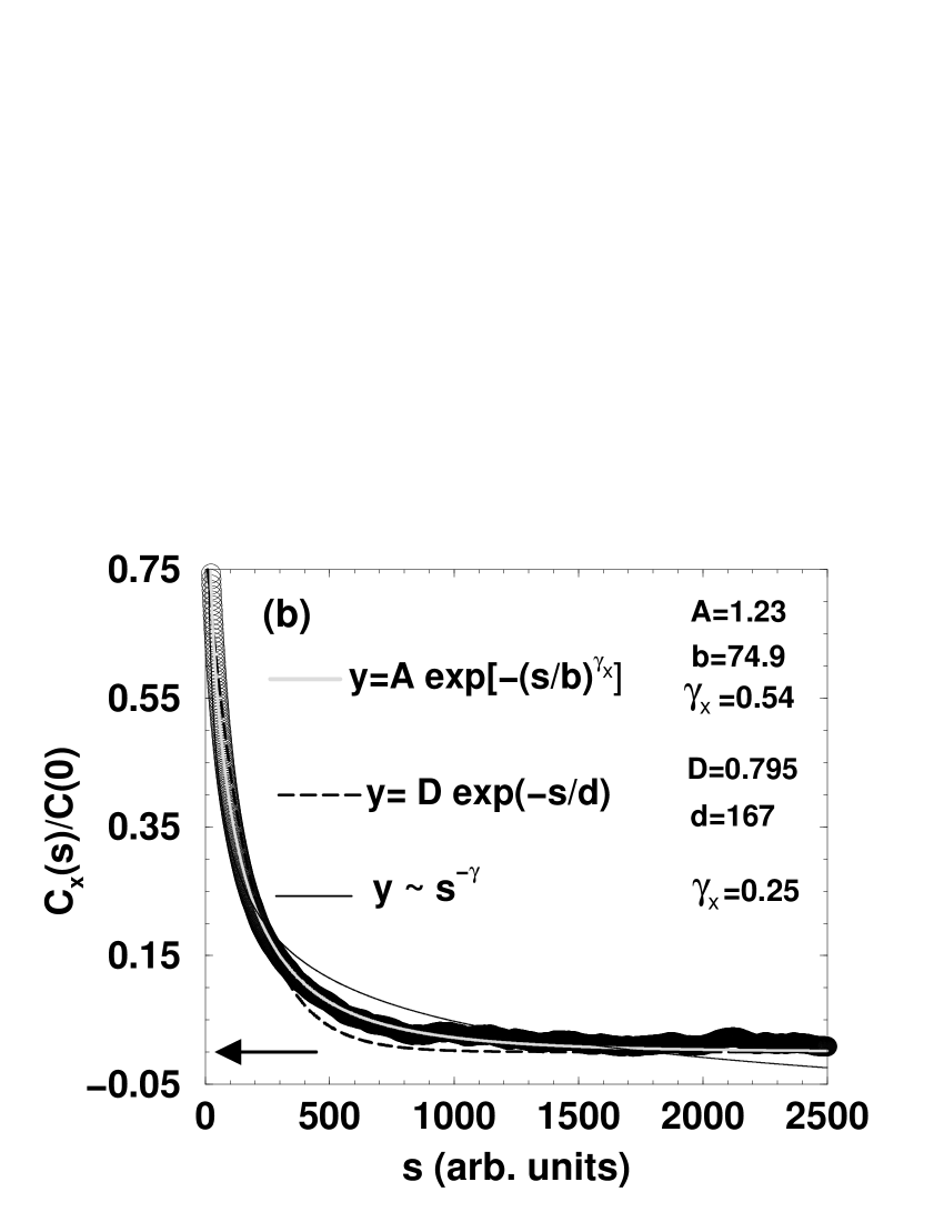
Figure 2: The black circles display the auto-correlation function, $C_{x}(s)$, of the signal in Fig. 1. $C_{x}$ has been normalized to $C_{x}(s=0)$. The black arrow at the bottom points out the origin on the y-axis. The grey curve represents the best-fit with a stretched exponential. The black curves, dashed and solid, show respectively the best-fit with an exponential and a power-law. The figure also reports the values of the best-fit parameters.

Figure 3: Return intervals of an extreme value above the threshold $q=4.5$ (in units of root-mean square deviation) for the time series in Fig. 1. The series consists of $1.6\times 10^{6}$ records. The values over the threshold are only $N_{q}=1781$ and the mean return period is $R_{q}=898$ (in simulation time-step units).

Figure 4: The same as Fig. 3 but obtained by shuffling the data (see the text).

Figure 5: Return intervals of an extreme value above the threshold $q=2.5$ (in units of root-mean square deviation) for the same time series considered in the previous figures. The values over the threshold now are $N_{q}=27268$ and the mean return period is $R_{q}=58.66$ (in simulation time-step units).

Figure 6: The same as Fig. 5 but obtained by shuffling the data (see the text).

Figure 7: Double-logarithmic plot of the probability density $P_{q}(r)$ of the return intervals distribution as a function of $r/R_{q}$ for different quantiles $q$. The probability densities have been normalized to $P_{q}(1)$. The slope of the straight line shown in the figure gives the value of the exponent $\gamma$ of a stretched exponential function fitting $P_{q}(r)$.

Figure 8: The same as Fig. 7 but obtained by shuffling the data.

Long $x(t)$ time series (typically made of $1\div 2\times 10^{6}$ records) have been generated and analyzed for different values of $\lambda$, of the external current and of the network size. The analysis has been performed by calculating the auto-correlation function $C_{x}$ and the PDF of the $x$ records, the return intervals $r_{q}$ of the extreme values for different threshold $q$ and their distribution $P_{q}(r)$. The values of $q$ are expressed in root-mean-square deviation units. At small $\lambda$ values (high level of intrinsic disorder), we have found that the auto-correlation function displays a non-exponential (but non-power-law) decay. This behavior is different from that displayed at high $\lambda$ values (low level of intrinsic disorder), where $C_{x}$ exhibits an exponential decay (consistent with the Lorentzian power spectrum reported in previous works [16, 17, 19]). Here we will focus on the case of non-exponential and non-power-law decay of correlations, a situation typical of systems which are approaching criticality, and we will show the results obtained by taking $\lambda=0.33$ for a network of size $125\times 125$, biased by a current $I=0.011$ A.

Figure 1 displays a portion of the $x(t)$ time series (the total number of records in $x(t)$ is $1.6\times 10^{6}$). The figure clearly shows a strong non-Gaussianity of the resistance fluctuations. Actually, with the above specified choice of the parameters, the PDF of the resistance fluctuations is well described by the Bramwell-Holdworth-Pinton [24] distribution, as discussed in Refs. [18, 19]. Figure 2 reports the auto-correlation function which significantly deviates from a single exponential or a power-law behavior. We have found that $C_{x}$ is well fitted by a stretched exponential function: $C_{x}(s)=A\$ exp$[(-s/b)^{\gamma})]$, with the following values of the fitting parameters: $A=1.23$, $b=74.9$ and $\gamma=0.54$. We have also considered many other functions for the best-fit of the $C_{x}$ data. However, we have found that the stretched exponential function optimizes the best-fit procedure with the minimum numbers of fitting parameters. We note that this expression of $C_{x}(s)$ recovers the simple exponential dependence for $\gamma=1$ while it provides a constant behavior for $\gamma=0$. Moreover, it provides a finite value of the average correlation time $\tau$. Figure 3 shows the return intervals of the extreme values above the threshold $q=4.5$. For comparison, in Fig. 4 we have reported the return intervals obtained for the same quantile by random shuffling the records of $x(t)$ (an operation which leaves unchanged the PDF of the x-data). The different scales of Fig. 3 and 4 must be underlined. Similarly to the results of Bunde et al. [5] concerning long-term correlated records, Fig. 3 shows a strong clustering of the extreme events: sequences of very short return intervals follow sequences of typically long intervals. This strong clustering is present even if the $x$ records are not long-term correlated while they are characterized by a finite correlation time. A situation completely different from that reported in Fig. 4, which corresponds to fully uncorrelated records. The clustering of extreme values persists also by lowering the threshold. This is displayed in Fig. 5 which shows the return intervals obtained for $q=2.5$. Again, Fig. 6 reports the returns intervals calculated by shuffling the x-data.

The probability density function $P_{q}(r)$ of the return intervals of extreme values is plotted in Fig. 7 in a double-logarithmic scale as a function of $r/R_{q}$ and for different quantiles $q$ (the probability density has been normalized to $P_{q}(1)$). This representation has been adopted for convenience: in fact in this plot a stretched exponential function with exponent $\gamma$ is represented by a straight line, whose slope just provides the value of $\gamma$. For check and comparison we have reported in Fig. 8 the probability density function $P_{q}(r)$ of the return intervals calculated after random shuffling the x-records: in this case $\gamma=1$, i.e. the distribution of the $r_{q}$ is exponential, as it must be for a Poisson process. Thus, Fig. 7 shows that the distribution of return intervals of extreme values of $x(t)$ is well described by a stretched exponential and that the value of the exponent $\gamma$ is independent of the threshold $q$ in a large range of $q$-values. Moreover, at least in the case of the data reported in Figs. 1-8, the value of the exponent $\gamma$ of the return interval distribution is just $1/2$ of the value of $\gamma_{x}$, the exponent of the auto-correlation function. An analysis performed on other sets of data, obtained for high disordered networks of different size $L$ and/or biased by different current density $I/L$, seems to confirm this last result. However, further investigations are necessary to establish the possible relationship between the two exponents.

3 Conclusions and Open Questions

We have studied the distribution of return intervals of extreme events in time series with finite-term correlations. Precisely, we have analyzed the auto-correlation function and the distribution of the return intervals of extreme values of the resistance fluctuations displayed by a resistor with granular structure in nonequilibrium stationary states. The resistance fluctuations were calculated by Monte Carlo simulations using the SBRN model [16, 17, 18, 19, 20]. We have found that for highly disordered networks, when the auto-correlation function displays a non-exponential (precisely, a stretched exponential) decay and the resistance fluctuations are characterized by a finite correlation time, the distribution of return intervals of the extreme values is well described by a stretched exponential with exponent $\gamma$ largely independent of the threshold $q$. Therefore our results show that the stretched exponential distribution [21] describes the distribution of return intervals of extreme events not only in the case of long-term correlated time series [3, 4, 5] but also when the records are characterized by finite-term correlations, with non-exponential decay of the auto-correlation function. Many open questions arise from this study and we limit to mention the following ones: i) why is the distribution of return intervals of extreme values a stretched exponential? what is the basic reason for this behavior which, as we have found, is not only limited to long-term correlated records [3, 4, 5] but is present also when non-exponential, finite term correlations are present? ii) what is the relationship between the exponents $\gamma$ and $\gamma_{x}$? The correlations among the $r_{q}$ have been studied in Refs. [3, 4, 5] in the case of long-term correlated processes, thus we can ask iii) what kind of correlations exist among the $r_{q}$ in the case of a finite-term, non-exponentially correlated processes ?

This work has been partially supported by the SPOT NOSED project IST-2001-38899 of E.C. and by the cofin-03 project ”Modelli e misure in nanostrutture” financed by Italian MIUR. The authors thank S. Ruffo (University of Florence, Italy), P. Olla (ISAC-CNR, Lecce, Italy) and G. Salvadori (University of Lecce, Italy) for helpful discussions.

References

- [1] H. von Storch and F. W. Zwiers. Statistical Analysis in Climate Research. Cambridge University Press, Cambridge, 2001.
- [2] S. Kotz and S. Nadarajah. Extreme Value Distributions, Theory and Applications. Imperial College Press, London, 2002.
- [3] E. G. Altmann and H. Kantz. Recurrence time analysis, long-term correlations, and extreme events. Phys. Rev. E, 71:056106–1–9, 2005.
- [4] A. Bunde, J. F. Eichner, S. Havlin, and J. W. Kantelhardt. The effect of long-term correlations on the return periods of rare events. Physica A, 330:1–7, 2003.
- [5] A. Bunde, J. F. Eichner, J. W. Kantelhardt, and S. Havlin. Long-term memory: a natural mechanism for the clustering of extreme events and anomalous residual times in climate records. Phys. Rev. Let., 94:048701–1–4, 2005.
- [6] A. Bunde, S. Havlin, J. W. Kantelhardt, T. Penzel, J.H. peter, and K. Voigt. Correlated and uncorrelated regions in heart-rate fluctuations during sleep. Phys. Rev. Lett., 85:3736–3739, 2000.
- [7] Y. Ashkenazy, P. C. Ivanov, S. Havlin, C. K. Peng, A. L. Goldberger, and H. E. Stanley. Magnitude and sign correlations in heartbeat fluctuations. Phys. Rev. Let., 86:1900, 2001.
- [8] J. Davidsen and H. G. Schuster. Simple model for 1/fα noise. Phys. Rev. E, 65:026120–1–4, 2002.
- [9] E. Koscielny-Bunde, A. Bunde, S. Havlin, H. E. Roman, Y. Goldreich, and H.J. Schellnhuber. Indication of a universal persistance law governing atmospheric variability. Phys. Rev. Lett., 81:729–732, 1998.
- [10] P. Bak, K. Christensen, L. danon, and T. Scanlon. Unified scaling law for earthquakes. Phys. Rev. Lett., 88:178501–1–4, 2002.
- [11] A. Corral. Long-term clustering, scaling, and universality in the temporal occurrence of earthquakes. Phys. Rev. Lett., 92:108501–1–4, 2004.
- [12] G. Boffetta, V. Carbone, P. Giuliani, P. Veltri, and A. Vulpiani. Power-laws in solar flares: self-organized criticality or turbulence? Phys. Rev. Lett., 83:4662–4665, 1999.
- [13] Y. Liu, P. Cizeau, M. Meyer, C. K. Peng, and H. E. Stanley. Correlations in economic time series. Physica A, 245:437–440, 1997.
- [14] M. Kac. -. Bull. of the Am. Math. Soc., 53:1002, 1947.
- [15] H. A. Makse, S. Havlin, M. Schwartz, and H. E. Stanley. Method for generating long-range correlations for large systems. Phys. Rev. E, 53:5445–5449, 1996.
- [16] C. Pennetta, L. Reggiani, G. Trefán, and E. Alfinito. Resistance and resistance fluctuations in random resistor networks under biased percolation. Phys. Rev. E, 65:066119–1–10, 2002.
- [17] C. Pennetta. Resistance noise near to electrical breakdown: steady state of random networks as a function of the bias. Fluct. and Noise Let., 2:R29–R49, 2000.
- [18] C. Pennetta, E.Alfinito, L. Reggiani, and S. Ruffo. Non-gaussian resistance noise near breakdown, in granular material. Physica A, 340:380–387, 2004.
- [19] C. Pennetta, E. Alfinito, L. Reggiani, and S. Ruffo. Non-gaussian resistance flutuations in disordered materials. In Z. Gingl, J. M. Sancho, L. Schimansky-Geier, and J. Kertesz, editors, Noise in Complex Systems and Stochastic Dynamics II, number 5471 in Proceedings of SPIE, pages 38–47, Bellingham, 2004. Int. Soc. Opt. Eng.
- [20] C. Pennetta, E. Alfinito, L. Reggiani, F. Fantini, I. de Munari, and A. Scorzoni. Biased resistor network model for electromigration failure and related phenomena in metallic lines. Phys. Rev. B, 70:174305–1–15, 2004.
- [21] D. Sornette. Critical Phenomena in Natural Sciences, Chaos, Fractals, Selforganization and Disorder: Concepts and Tools. Springer, Berlin, 2004.
- [22] C. Pennetta, G. Trefán, and L. Reggiani. A percolative approach to resistance fluctuations. In D. Abbott and L. B. Kish, editors, Unsolved Problems of Noise and Fluctuations, number 511 in AIP Conf. Proceedings, pages 447–452, New York, 1999. AIP.
- [23] C. Pennetta, L. Reggiani, and G. Trefán. Scaling law of resistance fluctuations in stationary random resistor networks. Phys. Rev. Let., 85:5238–5241, 2000.
- [24] S.T. Bramwell, P.C.W. Holdsworth, and J. F. Pinton. Universality of rare fluctuations in turbulence and critical phenomena. Nature, 396:552–554, 1998.