Avoided Crossings in Driven Systems

Abstract

We characterize the avoided crossings in a two-parameter, time-periodic system which has been the basis for a wide variety of experiments. By studying these avoided crossings in the near-integrable regime, we are able to determine scaling laws for the dependence of their characteristic features on the non-integrability parameter. As an application of these results, the influence of avoided crossings on dynamical tunneling is described and applied to the recent realization of multiple-state tunneling in an experimental system.

1 Introduction

Avoided crossings of eigenvalue curves are generic features of quantum systems with non-integrable classical counterparts [1]. Their appearance allows for a wide variety of interesting, purely quantum mechanical, phenomena including chaos-assisted tunneling [2], the adiabatic exchange of eigenstate character [3], and generally provides the mechanism by which underlying classical chaos affects the dynamics of a quantum system [4]. Their existence is also responsible for perhaps the most well-known result in the field of quantum chaos, the non-Poisson statistical distribution of level spacings in “chaotic” quantum systems [5].

In systems with two parameters, an avoided crossing along any curve in parameter space can be associated to a “diabolical point” at which two eigenvalue surfaces become degenerate [6]. The conical shape of the two eigenvalue surfaces in the vicinity of such a diabolical point ensures the characteristic hyperbolic behavior of two eigenvalues along any curve in parameter space passing near, but not through, the diabolical point. In the particular case of a near-integrable system, one parameter may be fixed to be zero leaving the system integrable for all values of the other parameter. Eigencurves will freely cross under variation of the latter parameter, thus creating diabolical points of the associated eigenvalue surfaces when viewed in the full two-parameter space. As we show here, this type of diabolical point is important because perturbation theory can be applied to characterize the conical shape and therefore characterize the avoided crossings of the near-integrable system.

In this paper we study the particular two-parameter, near-integrable system of a harmonically driven pendulum:

$$H(\kappa,\lambda)=p^{2}+\kappa\cos\theta+\lambda\left[\cos\left(\theta+\omega t\right)+\cos\left(\theta-\omega t\right)\right]\,.$$ (1)

This “one-and-a-half” degree-of-freedom system is one of the simplest types of classical systems to exhibit chaos. It is of significant experimental interest in quantum mechanics since it has been implemented in a number of studies [7, 8, 9, 10, 12] through the use of cold atom optics, particularly in investigations of multiple-state dynamical tunneling [12]. Theoretically, it provides a convenient framework for studying the avoided crossings of near-integrable systems since for $\lambda\rightarrow 0$ the system is the integrable pendulum Hamiltonian.

In the following, we study the properties of avoided crossings for the driven pendulum with the use of Floquet theory. An avoided crossing of two Floquet eigenvalue curves (for $\lambda\neq 0$) can be associated to a level crossing of the integrable pendulum ($\lambda=0$) system and is characterized by the dependence of its closest approach on the non-integrability parameter $\lambda$. For small values of $\lambda$, we find that the spacing exhibits a power law dependence with an integer power. A modified degenerate perturbation theory is then applied to verify this dependence and associate it to the direct or indirect coupling of the associated integrable eigenstates. We then use the perturbation results to elucidate a multiple state dynamical tunneling process in the vicinity of an avoided crossing and apply the results to the particular achievement of this tunneling in an atom optics experiment. We finally show the association of this avoided crossing to a nearby diabolical point.

In Section 2 we present the model Hamiltonian under consideration in the paper, including a description of the system’s classical dynamics. Section 3 presents the quantum dynamics of the model system, with a brief review of Floquet analysis. Avoided crossings of the model system are investigated in detail in Section 4, first numerically, then with the perturbation theory results presented in Appendix A. We review the implications of avoided crossings on dynamical tunneling in Section 5 and demonstrate the origin of those avoided crossings in a particular experimental system. Section 6 contains some concluding remarks.

2 The Model Hamiltonian

The Hamiltonian we consider consists of a particle moving in the presence of a harmonically-modulated, spatially-periodic potential. It can be written in the form

$$H^{\prime}(p^{\prime},x,t^{\prime})=\frac{{p^{\prime}}^{2}}{2m}+V_{1}\cos(kx)+V_{2}\cos(kx)\cos({\omega}^{\prime}t^{\prime}),$$ (2)

where $p^{\prime}$ is the momentum and $x$ the position of a particle of mass $m$, $t^{\prime}$ is time, $V_{1}$ is the amplitude of the spatially periodic potential, $V_{2}$ is the amplitude of the modulation potential and ${\omega}^{\prime}$ is the frequency of the modulation potential. The experimental implementation of quantum systems of with this type of Hamiltonian was first proposed by Graham, Schlautmann, and Zoller in 1992 [7] and then achieved by Raizen et. al. [8, 9, 12], and Hensinger et. al. [10].

It is useful to change to dimensionless units. We define: $p=\frac{p^{\prime}}{\hbar k}$, $\theta=kx$, $t=t^{\prime}\frac{E_{0}}{\hbar}$, $\omega=\omega^{\prime}\frac{\hbar}{E_{0}}$, $\kappa=\frac{V_{1}}{E_{0}}$, $\lambda=\frac{V_{2}}{2E_{0}}$, and $H=\frac{H^{\prime}}{E_{0}}$, where $E_{0}\equiv\frac{\hbar^{2}k^{2}}{2m}$. Then, the Hamiltonian in Eq. 2 takes the form

$$H(p,\theta,t)=H_{0}(p,\theta)+\lambda\left[\cos(\theta-{\omega}t)+\cos(\theta+{\omega}t)\right],$$ (3)

where

$$H_{0}(p,\theta)=p^{2}+\kappa\cos(\theta),$$ (4)

is the Hamiltonian of a pendulum and we have written the modulation term explicitly as two travelling waves. Note that momentum is measured in units of ${\hbar}k$.

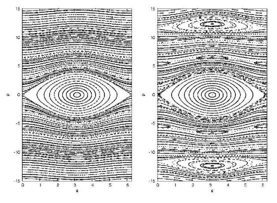
Figure 1: Strobe plots of the system in Eq. (3) with $\omega=24$ and parameters: (a) $\kappa=7.8$ and $\lambda=0$; and (b) $\kappa=7.8$ and $\lambda=1.0$.

The classical phase space of a time-periodic one-and-a-half degree-of-freedom system such as $H(p,\theta,t)$ can be visualized by a strobe plot of the trajectories at times $t=\nu\frac{2\pi}{\omega}\;\;(\nu\in Z)$. A strobe plot of phase space trajectories for the system governed by Hamiltonian $H(p,\theta,t)$ is shown in Figure 1.a with parameters $\kappa=7.8$ and $\lambda=0$. (For the case of $\lambda=0$, the system is independent of time and could be visualized with an ordinary parametric plot of phase space, however we plot the strobed phase space for convenience of comparison to the perturbed system). Because this system is integrable, all orbits lie on tori (in either the regions of the pendulum’s libration or rotation) and the phase space is absent of chaos. Figure 1.b shows a strobe plot of the phase space with parameters $\kappa=7.8$, $\lambda=0.5$, and $\omega=24$. The travelling waves in the modulation term have phase velocities $v=\pm\omega$ and are seen as primary resonance structures at $p=\pm\frac{\omega}{2}$ where $\dot{\theta}=v$. Although much of the orbit structure of the integrable system is preserved, the tori with rational winding numbers have been destroyed, giving rise to a self-similar set of daughter resonance structures (see, for example, the two-island chains at $p=\pm\frac{\omega}{4}$). Regions of chaos surround these resonances, most visibly near the separatrix of the pendulum resonance.

3 Quantum Dynamics

The dimensionless Schrödinger equation for the system in Eq. (3) is $i\frac{\partial}{\partial t}|{\psi}(t)\rangle=\hat{H}(t)|{\psi}(t)\rangle$, where

$$\quad\quad\hat{H}(t)=\hat{p}^{2}+\kappa\cos\hat{\theta}+2\lambda\cos\left(\hat{\theta}\right)\,\cos(\omega t)\,,$$ (5)

We will consider the configuration space, $\theta\in[0,2\pi)$, to be periodic such that $\langle\theta+2\pi|\psi(t)\rangle=\langle\theta|\psi(t)\rangle$ and the momentum operator has integer eigenvalues: $\hat{p}|p\rangle=n|p\rangle\;\;(n\in Z)$. In the experimental systems, this is approximately achieved naturally because momentum transfer occurs in discrete units of $\hbar k$ [9, 10, 11].

When $\lambda=0$, the Hamiltonian reduces to that of the quantum pendulum, $\hat{H}_{0}(\kappa)=\hat{p}^{2}+\kappa\cos\hat{\theta}$. The eigenstates of $\hat{H}_{0}$ are Mathieu functions [13] which we will henceforth denote as $|n(\kappa)\rangle$ so that $\hat{H}_{0}(\kappa)|n(\kappa)\rangle=E_{n}(\kappa)|n(\kappa)\rangle$ where $n=0,\pm 1,\pm 2,\ldots$. (We will suppress the $\kappa$-dependence of these eigenstates until their specification is necessary). States $|n\rangle$ with positive integer labels are those with even parity, states with negative integer label are those with odd parity. Note that as $\kappa\rightarrow 0$, $E_{n}\rightarrow n^{2}$. If $\kappa\neq 0$, but $|n|$ is large (i.e. the corresponding classical pendulum energy is much larger than that of the separatrix), we will again have $E_{n}\approx n^{2}$.

3.1 Floquet Theory

The Hamiltonian in Eq. (5) is time-periodic and therefore Floquet’s theorem guarantees that solutions of the Schrödinger equation can be written in the form

$$|\psi_{\alpha}(t)\rangle={\rm e}^{-i\Omega_{\alpha}t}|\phi_{\alpha}(t)\rangle\quad{\rm with}\quad|\phi_{\alpha}(t+T)\rangle=|\phi_{\alpha}(t)\rangle\,,$$ (6)

where we have defined $T=\frac{2\pi}{\omega}$ and where $|\phi_{\alpha}(t)\rangle$ and $\Omega_{\alpha}$ are called the Floquet eigenstate and eigenvalue, respectively. Substituting this solution into the Schrödinger equation yields the eigenvalue equation

$$\hat{H}_{F}(t)|\phi_{\alpha}(t)\rangle\equiv\left(\hat{H}(t)-i\frac{\partial}{\partial t}\right)|\phi_{\alpha}(t)\rangle=\Omega_{\alpha}|\phi_{\alpha}(t)\rangle\,,$$ (7)

where $\hat{H}_{F}(t)$ is called the Floquet Hamiltonian.

The Floquet Hamiltonian is a Hermitian operator in a composite Hilbert space $\Theta\otimes\mathcal{T}$ [14, 15], where $\Theta$ is the space of all square-integrable functions $f(\theta)$ on the configuration space and $\mathcal{T}$ is the space of all time-periodic functions $a(t)$ with period $T$ and finite $\int_{-T/2}^{T/2}|a(t)|^{2}dt$. The inner product of two vectors $|\phi_{a}\rangle$ and $|\phi_{b}\rangle$ in this space is then defined by

$$\langle\langle\phi_{a}|\phi_{b}\rangle\rangle\equiv\frac{1}{T}\int_{-T/2}^{T/2}\langle\phi_{a}|t\rangle\langle t|\phi_{b}\rangle dt=\frac{1}{T}\int_{-T/2}^{T/2}\langle\phi_{a}(t)|\phi_{b}(t)\rangle dt\,,$$ (8)

where $\langle\phi_{a}(t)|\phi_{b}(t)\rangle=\int_{0}^{2\pi}\langle\phi_{a}(t)|\theta\rangle\langle\theta|\phi_{b}(t)\rangle d\theta$ is the usual inner product in $\Theta$. We select a complete orthonormal basis in this composite space

$$\langle t|n,q\rangle=|n\rangle\;{\rm e}^{iq\omega t}\quad\quad\left(n,q\in Z\right)\,,$$ (9)

where $\left\{|n\rangle\right\}$ are the eigenstates of the pendulum Hamiltonian $\hat{H}_{0}$. These basis vectors satisfy $\langle\langle n,q|n^{\prime},q^{\prime}\rangle\rangle=\delta_{n,n^{\prime}}\delta_{q,q^{\prime}}$.

The Floquet Hamiltonian $\hat{H}_{F}$ is Hermitian, so the Floquet eigenvalues $\Omega_{\alpha}$ are real and two Floquet eigenstates $|\phi_{\alpha}\rangle$ and $|\phi_{\beta}\rangle$ belonging to different eigenvalues are orthogonal. Additionally, the Floquet Hamiltonian commutes with the parity operator defined by its action on the momentum eigenket $\hat{\Pi}|p\rangle=|-p\rangle$. Therefore the two operators can be diagonalized simultaneously and all Floquet eigenstates have definite parity: $\hat{\Pi}|\phi_{\alpha}\rangle=\pm 1|\phi_{\alpha}\rangle$. Floquet states with parity eigenvalue $+1$ will be called even, those with eigenvalue $-1$ odd.

Given one Floquet eigenstate $|\phi_{\alpha}(t)\rangle$ with Floquet eigenvalue $\Omega_{\alpha}$, there will be another Floquet eigenstate $|\phi^{\prime}_{\alpha}(t)\rangle$ such that $|\phi^{\prime}_{\alpha}(t)\rangle\equiv{\rm e}^{iq\omega t}|\phi_{\alpha}(t)\rangle\;\;(q\in Z)$, with eigenvalue $\Omega_{\alpha}^{\prime}\equiv\Omega_{\alpha}+q\omega$. These two Floquet eigenstates, however, represent the same physical state, i.e.

$${\rm e}^{-i\Omega^{\prime}_{\alpha}t}|\phi^{\prime}_{\alpha}(t)\rangle={\rm e}^{-i\Omega_{\alpha}t}|\phi_{\alpha}(t)\rangle\,.$$ (10)

Therefore we may limit consideration to the fundamental zone $-\omega/2\leq\Omega<\omega/2$ in which each physical eigenstate of the time-dependent Schrödinger equation is represented by the corresponding Floquet eigenstate with eigenvalue within that range.

Consider the unperturbed system $\hat{H}_{F}^{0}\equiv\hat{H}_{0}-i\frac{\partial}{\partial t}$ which we will call the Floquet pendulum. The eigenstates of this system are precisely the basis states $|n,q\rangle$ with eigenvalues $\Omega_{nq}=E_{n}+q\omega$. Figure 2 shows the lowest nine energies of the even-parity eigenstates of the quantum pendulum and the corresponding Floquet eigenvalues in the fundamental zone $-\omega/2\leq\Omega<\omega/2$.

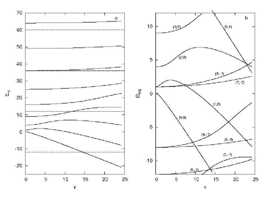
Figure 2: (a) Energy curves of the nine lowest-energy, even-parity eigenstates of the quantum pendulum, $\hat{H}_{0}=\hat{p}^{2}+\kappa\cos\hat{\theta}$. (b) The nine corresponding “Floquet pendulum” eigenvalues in the fundamental zone $-\frac{\omega}{2}<{\Omega}\leq+\frac{\omega}{2}$ with $\omega=24$. The labels $(n,q)$ on each Floquet eigenvalue segment identify the corresponding Floquet eigenstate $|n,q\rangle$. The dashed lines in (a) indicate the Floquet eigenvalue zone boundaries.

3.2 Another method for determining Floquet states

An arbitrary dynamical state of the system can be expanded, with the use of equation (6), in the basis of Floquet eigenstates,

$$|\psi(t)\rangle={\sum_{\alpha}}^{\prime}A_{\alpha}{\rm e}^{-i\Omega_{\alpha}t}|\phi_{\alpha}(t)\rangle\,,$$ (11)

where the “prime” indicates that the sum is restricted to those Floquet states with $\Omega_{\alpha}$ in the fundamental zone. The expansion coefficients are independent of time and can be written $A_{\alpha}=\langle\phi_{\alpha}(0)|\psi(0)\rangle$. Using the time-periodicity of the Floquet eigenstates, we can then write

$$|\psi(T)\rangle=\sum_{\alpha}^{\prime}{\rm e}^{-i\Omega_{\alpha}T}|\phi_{\alpha}(0)\rangle\langle\phi_{\alpha}(0)|\psi(0)\rangle\equiv\hat{\rm U}(T)|\psi(0)\rangle\,,$$ (12)

showing that the time-evolution operator over a single period $T$

$$\hat{\rm U}(T)={\sum_{\alpha}}^{\prime}{\rm e}^{-i\Omega_{\alpha}T}|\phi_{\alpha}(0)\rangle\langle\phi_{\alpha}(0)|$$ (13)

is diagonalized by the Floquet eigenstates at time $t=0$. We can therefore determine these time-strobed Floquet states by constructing the matrix ${\rm U}_{mm^{\prime}}\equiv\langle m|\hat{\rm U}(T)|m^{\prime}\rangle$ in some convenient basis $\{|m\rangle\}$ in $\Theta$, truncating this matrix at some appropriate level $m=M$ where it becomes approximately diagonal (i.e. ${\rm U}_{MM}>>{\rm U}_{Mm}$ for $m\neq M$), and then performing a numerical diagonalization to obtain the $|\phi_{\alpha}(0)\rangle$ and $\Omega_{\alpha}$ (mod $\omega$). The $m^{th}$ column of ${\rm U}$ is obtained by evolving the basis vector $|m\rangle$ over one period $T$ via numerical integration of the Schrödinger equation.

In subsequent sections, we will compare the phase space distributions of the time-strobed Floquet eigenstates $|\phi_{\alpha}(0)\rangle$ to the classical system. We can do this by introducing the Husimi distribution $\rho(\theta_{0},p_{0})$ [16, 17] of a quantum state $|\phi\rangle$ on the classical phase space $(\theta_{0},p_{0})$

$$\rho(\theta_{0},p_{0})\equiv\frac{1}{2\pi}|\langle\theta_{0},p_{0}|\phi\rangle|^{2}\,,$$ (14)

where the coherent state $|\theta_{0},p_{0}\rangle$ is defined as an eigenstate of the annihilation operator $\hat{a}=\frac{1}{\sqrt{2}}\left(\hat{\theta}/{\sigma}+i\sigma\hat{p}\right)$ with position and momentum expectation values of $\theta_{0}$ and $p_{0}$ respectively. The free parameter $\sigma$ is set according to the physical system considered (see below). The representation of such a coherent state in the discrete momentum basis $\{|p\rangle\}$ is given by

$$\langle p|\theta_{0},p_{0}\rangle=A\exp\left[-\frac{\sigma^{2}}{2}(p-p_{0})^{2}-i\theta_{0}(p-p_{0})\right]\,,$$ (15)

where $A$ is a normalization factor guaranteeing $\langle\theta_{0},p_{0}|\theta_{0},p_{0}\rangle=1$. The action of the annihilation operator on the coherent state can be used to show that $\langle p\rangle\equiv\langle\theta_{0},p_{0}|\hat{p}|\theta_{0},p_{0}\rangle=p_{0}$, $\langle\theta\rangle=\theta_{0}$, $\Delta\theta=\sigma/\sqrt{2}$, and $\Delta p=(\sigma\sqrt{2})^{-1}$. Thus, the coherent state is a minimum-uncertainty wavepacket, where the free parameter determines the ratio of its uncertainty in position and momentum, i.e. $\sigma^{2}=\Delta\theta/\Delta p$. Reference [17] presents an in-depth discussion on the selection of the parameter $\sigma$. In all Husimi plots shown in subsequent sections, we set $\sigma=1.18\,\kappa^{-1/4}$, a choice which provides the best association between the quantum pendulum eigenfunctions and the corresponding classical orbits). As we will see, the Husimi distributions of the Floquet states lie directly on the orbit structures of the classical phase space.

4 Avoided crossings

The Floquet pendulum is integrable and its eigenvalues $\Omega_{n,q}(\kappa)$, shown in Figure 2.b, cross under the variation of $\kappa$. For any nonzero $\lambda$, however, the system represented by the Hamiltonian in Eq. (5) is non-integrable and the approach of any two (same parity) Floquet eigenvalues under variation of $\kappa$ results in an avoided crossing. This well-known result, the no-crossing theorem, was first proven by von Neumann and Wigner for eigenvalues of generic Hermitian matrices [1]. They also showed that adiabatic passage of two quantum states through an avoided crossing leads to an exchange of character. (In a two-parameter system, this exchange can be related to the partial circuit of a diabolical point [6], while in single parameter systems it can be related to exceptional points in the complex parameter plane [18]). Avoided crossings of Floquet eigenvalues in the fundamental zone, which generally involve states localized in well-separated regions of the phase space, will therefore allow a wide variety of interesting quantum dynamical phenonomena, including adiabatic transitions and tunneling.

In this section, we will consider the near-integrable regime ($0<\lambda<<\kappa$), in which a clear association can be made between the Floquet eigenstates of the perturbed system ($\lambda\neq 0$) and those of the Floquet pendulum ($\lambda=0$). In this regime, the Floquet eigenvalues will follow nearly the same dependence on $\kappa$ as the unperturbed eigenvalues seen in Figure 2.b, except in the vicinity of an avoided crossing. For $\kappa$ values sufficiently far from these avoided crossings, we can make a unique, though necessarily local, association $|\phi_{\alpha}\rangle\leftrightarrow|n_{\alpha},q_{\alpha}\rangle$ of the Floquet eigenstate $|\phi_{\alpha}\rangle$ to the Floquet pendulum state with maximum overlap $|\langle n,q|\phi_{\alpha}\rangle|$. As $\lambda\rightarrow 0$, this association will become an equality. We will see that the fundamental characteristics of an avoided crossing between states $|\phi_{\alpha}\rangle$ and $|\phi_{\beta}\rangle$ will be determined by the difference

$$\Delta q_{\alpha\beta}\equiv|q_{\alpha}-q_{\beta}|\,.$$ (16)

In the subsections below, we first present a numerical analysis of some representative avoided crossings in the system with $\omega=24$, and then use perturbation theory to show that the results are quite general.

4.1 Numerical Results

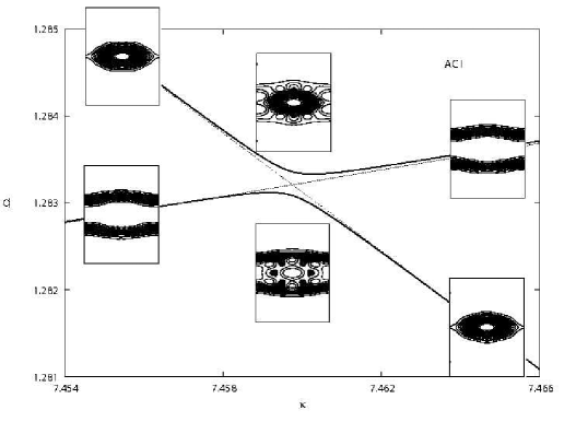
Figure 3: A $\Delta q_{\alpha\beta}=1$ avoided crossing of the system $\hat{H}_{F}$ with parameters $\omega=24$ and $\lambda=5\times 10^{-2}$. The Husimi distributions of the corresponding Floquet eigenstates are shown at $\kappa=(7.455,7.460,7.465)$ (the horizontal axis is $\theta_{0}\in[0,2\pi)$, vertical is $p_{0}\in[-15,15]$). The dotted lines are the eigencurves of the unperturbed Floquet pendulum.

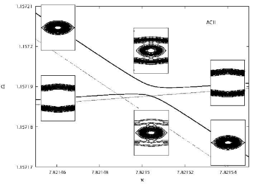
Figure 4: A $\Delta q_{\alpha\beta}=2$ avoided crossing of the system $\hat{H}_{F}$ with the same $\lambda$ and $\omega$ values as in Figure 3. The Husimi distributions shown are the two Floquet eigenstates at $\kappa=(7.82146,7.82150,7.82154)$ (axes are the same as Figure 3). The dotted lines are the eigencurves of the unperturbed Floquet pendulum.

Figure 5: A $\Delta q_{\alpha\beta}=3$ avoided crossing of the system $\hat{H}_{F}$ with the same $\lambda$ and $\omega$ values as in Figure 3. The Husimi distributions shown are the two Floquet eigenstates at $\kappa=(9.973221751,9.9732217534,9.973221755)$ (axes are the same as Figure 3). The crossing of the corresponding eigencurves of the unperturbed Floquet pendulum falls outside of the plotted region at $\kappa_{0}\approx 9.973242$.

Three avoided crossings of Floquet eigenvalues in the fundamental zone with $\lambda=5\times 10^{-2}$ are shown in Figures 3, 4, and 5 with Husimi plots of the corresponding Floquet eigenstates overplotted on the figures. The dotted lines shown are the eigenvalues of the unperturbed Floquet pendulum. These plots were created by numerically calculating the time-strobed Floquet states at a sequence of $\kappa$ values. With each step forward in $\kappa$, the new states were associated to those of the previous step by calculating the maximum overlap and verifying continuity of the eigenvalues. In the case that two Floquet eigenvalues crossed between $\kappa$-steps, the size of the step was reduced and the process repeated until no crossing occurred.

Each of these three avoided crossings involves one Floquet eigenstate localized within the pendulum resonance at $p=0$ and another localized outside of the pendulum resonance. The avoided crossing in Figure 3 involves the states $(n_{\alpha},q_{\alpha})=(1,0)$ and $(n_{\beta},q_{\beta})=(5,-1)$; Figure 4 involves the states $(n_{\alpha},q_{\alpha})=(1,0)$ and $(n_{\beta},q_{\beta})=(7,-2)$; and Figure 5 involves states $(n_{\alpha},q_{\alpha})=(0,0)$ and $(n_{\beta},q_{\beta})=(8,-3)$. The associated crossings can be found in Figure 2.b. These particular avoided crossings were chosen as representative examples with $\Delta q_{\alpha\beta}=1$, $2$, and $3$, respectively.

Some general characteristics of these avoided crossings deserve attention. First, the “exchange of character” between the two states is evident in the evolution of the Husimi distributions with $\kappa$. The associations $|\phi_{\alpha}\rangle\leftrightarrow|n_{\alpha},q_{\alpha}\rangle$ and $|\phi_{\beta}\rangle\leftrightarrow|n_{\beta},q_{\beta}\rangle$ well before the avoided crossing become $|\phi_{\alpha}\rangle\leftrightarrow|n_{\beta},q_{\beta}\rangle$ and $|\phi_{\beta}\rangle\leftrightarrow|n_{\alpha},q_{\alpha}\rangle$ well after. For $\kappa$ values at the avoided crossing, the two Floquet states are superpositions of the asymptotic states. Second, there is quite a disparity of scale among the three avoided crossings. In particular, the minimum eigenvalue spacing $\Delta_{\alpha\beta}$, defined by

$$\Delta_{\alpha\beta}\equiv{\rm min}\left(|\Omega_{\alpha}-\Omega_{\beta}|\right)\,,$$ (17)

is relatively large for the first and relatively small for the third. Finally, the position $\kappa_{ac}$ of the minimum spacing (which we will henceforth call the “position of the avoided crossing”), is not necessarily equal to the position $\kappa_{0}$ of the unperturbed crossing. Indeed, it seems that for $\Delta q_{\alpha\beta}\neq 1$, the avoided crossing is significantly offset in both $\kappa$ and $\Omega$.

Figure 6: The minimum spacing $\Delta_{\alpha\beta}$ as a function of $\lambda$ of the three avoided crossings shown in Figures 3, 4, and 5. The functions $\Delta_{\alpha\beta}=5.44\times 10^{-3}\lambda$, $\Delta_{\alpha\beta}=1.02\times 10^{-3}\lambda^{2}$, $\Delta_{\alpha\beta}=7.35\times 10^{-7}\lambda^{3}$ are overplotted.

To make these last two observations more quantitative, we have computed dependence of $\Delta_{\alpha\beta}$ and $\Delta\kappa_{ac}\equiv|\kappa_{0}-\kappa_{ac}|$ on the parameter $\lambda$. The results for the three example avoided crossings are shown in Figures 6 and 7. We see that, for small values of $\lambda$, the dependences are all well approximated by power laws with integer exponents. The minimum spacing of the avoided crossings is given by

$$\Delta_{\alpha\beta}=A\;\lambda^{\Delta q_{\alpha\beta}}\,,$$ (18)

where the coefficients are $A\approx\{5.44\times 10^{-3},1.02\times 10^{-3},7.35\times 10^{-7}\}$ for avoided crossings I,II, and III, respectively. The $\kappa$-offset of the avoided crossings are given by

$$\Delta\kappa_{ac}=B\;\lambda^{2}\,,$$ (19)

where $B\approx\{5.2\times 10^{-3},-8.3\times 10^{-3}\}$ for avoided crossings II and III ($\Delta\kappa_{ac}=0$ for avoided crossing I).

Figure 7: The $\kappa$-offset $\Delta\kappa_{ac}$ as a function of $\lambda$ for the avoided crossings shown in Figures 4 and 5. The functions $|\Delta\kappa_{ac}|=5.2\times 10^{-3}\;\lambda^{2}$ and $|\Delta\kappa_{ac}|=8.3\times 10^{-3}\;\lambda^{2}$ are overplotted.

4.2 Perturbation theory results

We now use perturbation theory to determine the behavior of the Floquet eigenvalues and eigenstates in the neighborhood of avoided crossings. We will obtain approximate solutions ($|\phi_{\alpha}\rangle,\Omega_{\alpha}$) to the Floquet eigenvalue equation

$$\hat{H}_{F}(\kappa,\lambda)|\phi_{\alpha}(\kappa,\lambda)\rangle=\left(\hat{H}^{0}_{F}(\kappa)+\lambda\hat{V}\right)|\phi_{\alpha}(\kappa,\lambda)\rangle=\Omega_{\alpha}(\kappa,\lambda)|\phi_{\alpha}(\kappa,\lambda)\rangle\,,$$ (20)

where $\hat{H}^{0}_{F}(\kappa)$ is the Floquet pendulum Hamiltonian, $\hat{V}=2\cos\hat{\theta}\,\cos(\omega t)$, and $\lambda$ is considered a small expansion parameter. Our unperturbed system is the two-fold degenerate system $\hat{H}^{0}_{F}(\kappa_{0})$, where $\kappa_{0}$ is the parameter value at which the eigenvalue curves of two Floquet pendulum states $|\alpha^{0}(\kappa)\rangle\equiv|n_{\alpha},q_{\alpha}\rangle$ and $|\beta^{0}(\kappa)\rangle\equiv|n_{\beta},q_{\beta}\rangle$ cross. We have seen in Section 4.1 that, for $\lambda\neq 0$, the closest approach of the eigenvalues $\Omega_{\alpha}$ and $\Omega_{\beta}$ involved in an avoided crossing may not occur at $\kappa=\kappa_{0}$, so an offset must be allowed for. We therefore introduce into (20) an arbitrary function $\kappa(\lambda)=\kappa_{0}+\Delta\kappa(\lambda)$ and expand $\Delta\kappa(\lambda)$ as a power series in $\lambda$. The particular value $\kappa_{ac}(\lambda)$ at which the eigenvalues make their closest approach can then be determined by solving the extremal condition for $\Delta\Omega_{\alpha\beta}\equiv|\Omega_{\alpha}(\kappa,\lambda)-\Omega_{\beta}(\kappa,\lambda)|$,

$$\left.\frac{\partial\Delta\Omega_{\alpha\beta}}{\partial\kappa}\right\rvert_{\kappa=\kappa_{ac}}=0\,,$$ (21)

at each order to fix the expansion coefficients of $\Delta\kappa(\lambda)$. In this manner, we find the perturbed eigenstates and eigenvalues at $\kappa=\kappa_{ac}$.

The details of the perturbation analysis are given in Appendix A. The results may be summarized as follows. The breaking of the degeneracy between states $|\alpha^{0}\rangle$ and $|\beta^{0}\rangle$ occurs at the lowest order $\lambda^{N}$ for which the coupling between these states, $v^{(N)}_{\alpha\beta}$ (defined below), is nonzero. At this order, the two Floquet eigenvalues in the region of the avoided crossing are determined by the eigenproblem of a $2\times 2$ matrix in the basis of the unperturbed states $|\alpha^{0}(\kappa_{0})\rangle$ and $|\beta^{0}(\kappa_{0})\rangle$:

$$\left(\begin{array}[]{cc}\Delta\kappa^{(N)}{\delta}E_{\alpha}+v^{(N)}_{\alpha\alpha}&v^{(N)}_{\alpha\beta}\\ v^{(N)}_{\beta\alpha}&\Delta\kappa^{(N)}{\delta}E_{\beta}+v^{(N)}_{\beta\beta}\end{array}\right)\left(\begin{array}[]{c}C^{\pm}_{\alpha}\\ C^{\pm}_{\beta}\\ \end{array}\right)=\Omega_{\pm}^{(N)}\left(\begin{array}[]{c}C^{\pm}_{\alpha}\\ C^{\pm}_{\beta}\\ \end{array}\right)\,.$$ (22)

The coefficients $C^{\pm}_{\alpha}$ and $C^{\pm}_{\beta}$ determine the zeroth-order near-degenerate eigenstates in the region of the avoided crossing; $\Delta\kappa^{(N)}$ and $\Omega_{\pm}^{(N)}$ are the coefficients of $\lambda^{N}$ in the expansions of the arbitrary $\kappa$-offset and the near-degenerate Floquet eigenvalues $\Omega_{\pm}$, respectively; $\delta E_{i}=\langle n_{i}(\kappa_{0})|\cos{\theta}|n_{i}(\kappa_{0})\rangle$ are the slopes of the unperturbed eigencurves; and $v^{(N)}_{ij}$ depends on the matrix elements of the perturbation operator:

$$V_{lm}\equiv\langle\langle n_{l},q_{l}|\hat{V}|n_{m},q_{m}\rangle\rangle=\langle n_{l}(\kappa_{0})|\cos\hat{\theta}|n_{m}(\kappa_{0})\rangle\left(\delta_{q_{l},q_{m}+1}+\delta_{q_{l},q_{m}-1}\right)\,.$$ (23)

For the first three orders in $\lambda$, these couplings are

$$v_{ij}^{(1)}=V_{ij}$$ (24)

$$v_{ij}^{(2)}=\sum_{\gamma\not\in\{\alpha,\beta\}}\frac{V_{i\gamma}V_{\gamma j}}{\Omega^{(0)}-\Omega^{(0)}_{\gamma}}$$ (25)

$$v_{ij}^{(3)}=\sum_{\gamma\not\in\{\alpha,\beta\}}\left\{\sum_{\sigma\not\in\{\alpha,\beta\}}\frac{V_{i\gamma}V_{\gamma\sigma}V_{\sigma j}}{\left(\Omega^{(0)}-\Omega^{(0)}_{\gamma}\right)\left(\Omega^{(0)}-\Omega^{(0)}_{\sigma}\right)}\right.$$

$$\left.+\delta_{ij}\frac{V_{i\gamma}V_{\gamma i}\left[V_{\alpha\alpha}(\delta E_{\alpha}-\delta E_{\gamma})+V_{\beta\beta}\left(\delta E_{\gamma}-\delta E_{\beta}\right)\right]}{\left(\Omega^{(0)}-\Omega^{(0)}_{\gamma}\right)^{2}}\right\}\,,$$ (26)

where $i,j\in\{\alpha,\beta\}$, the zeroth-order eigenvalues $\Omega^{(0)}_{l}$ are taken at $\kappa_{0}$, and we write $\Omega^{(0)}=\Omega_{\pm}^{(0)}$. Using Eqs. (22) and (21) we find that the $N^{th}$-order corrections to the eigenvalues, at the position of the avoided crossing, are given by

$$\begin{split}\Omega^{(N)}_{\pm}(\kappa_{ac})&=\frac{1}{2}\left[v_{\alpha\alpha}^{(N)}+v_{\beta\beta}^{(N)}+\Delta\kappa^{(N)}_{ac}\left(\delta E_{\alpha}+\delta E_{\beta}\right)\right]\\ &\quad\pm\frac{1}{2}\sqrt{\left[v_{\alpha\alpha}^{(N)}-v_{\beta\beta}^{(N)}+\Delta\kappa^{(N)}_{ac}\left(\delta E_{\alpha}-\delta E_{\beta}\right)\right]^{2}+4|v_{\alpha\beta}^{(N)}|^{2}}\\ &=\frac{v^{(N)}_{\beta\beta}-v^{(N)}_{\alpha\alpha}}{\delta E_{\alpha}-\delta E_{\beta}}\pm|v^{(N)}_{\alpha\beta}|\,.\end{split}$$ (27)

At orders $0<M<N$, the two eigenvalues $\Omega_{\pm}$ are degenerate at an offset from $(\kappa_{0},\Omega^{(0)})$ specified by the coefficients

$$\Delta\kappa^{(M)}=\frac{v^{(M)}_{\beta\beta}-v^{(M)}_{\alpha\alpha}}{\delta E_{\alpha}-\delta E_{\beta}}\,,$$ (28)

and

$$\Omega^{(M)}=\frac{v^{(M)}_{\beta\beta}\delta E_{\alpha}-v^{(M)}_{\alpha\alpha}\delta E_{\beta}}{\delta E_{\alpha}-\delta E_{\beta}}\,.$$ (29)

The origin of the numerical results presented in section 4.1 is now clear. The matrix elements of the perturbation $V_{ij}$ are non-zero only when $\Delta q_{ij}=1$. Therefore, for an avoided crossing between states $|\phi_{\alpha}\rangle$ and $|\phi_{\beta}\rangle$, we must have $\Delta q_{\alpha\beta}=N$. Using Eq. (27) and the fact that $\Omega^{(M<N)}$ is the same for $|\phi_{\alpha}\rangle$ and $|\phi_{\beta}\rangle$, we find that, to lowest order in $\lambda$, the minimum spacing is given by

$$\Delta_{\alpha\beta}=2\;\left\lvert\,v^{(\Delta q_{\alpha\beta})}_{\alpha\beta}\right\rvert\;\lambda^{\Delta q_{\alpha\beta}}\,.$$ (30)

Its interesting to note that the $\kappa$-offset of an avoided crossing in this system is dependent on $\lambda^{2}$, because $v^{(2)}_{\alpha\alpha}$ and $v^{(2)}_{\beta\beta}$ are non-zero, even when $\Delta q_{\alpha\beta}>2$.

$$\begin{array}[]{|l|l|l|l|l|l|l|l|}\hline\cr\kappa_{ac}&(n_{\alpha},q_{\alpha})&(n_{\beta},q_{\beta})&\Delta q_{\alpha\beta}&A_{\rm num}&A_{\rm pt}&B_{\rm num}&B_{\rm pt}\\ \hline\cr 7.46&(1,0)&(5,-1)&1&5.44\times 10^{-3}&5.5\times 10^{-3}&~{}~{}~{}---&~{}~{}~{}---\\ 7.83&(1,0)&(7,-2)&2&1.02\times 10^{-3}&1.0\times 10^{-3}&5.2\times 10^{-3}&5.2\times 10^{-3}\\ 9.97&(0,0)&(8,-3)&3&7.35\times 10^{-7}&7.3\times 10^{-7}&-8.3\times 10^{-3}&-8.3\times 10^{-3}\\ \hline\cr\end{array}$$

Table 1: Comparison of numerical results to those of perturbation theory. The quantities $A_{\rm num}$ and $B_{\rm num}$ are obtained from numerical simulation and $A_{\rm pt}$ and $B_{\rm pt}$ are obtained from perturbation theory.

Table 1 shows a quantitative comparison of the numerical results presented in the previous section (in terms of the coefficients $A$ and $B$ of Eqs. (18) and (19)) to those obtained by the perturbation analysis. For all three examples of avoided crossings, we see excellent agreement. We have also verified the predictions of perturbation theory for a number of other avoided crossings in this system (as well as those in systems with different values of $\omega$), finding similar agreement.

A number of other characteristics of the avoided crossings can be determined from our perturbation analysis. Substituting $\Omega^{(N)}_{\pm}(\kappa_{ac})$ and $\Delta\kappa^{(N)}_{ac}$ into Eq. (22), we find that at the position of the avoided crossing, the two perturbed Floquet eigenstates (to lowest order in $\lambda$) become an equal superposition of the two associated Floquet pendulum states, i.e.

$$|C^{\pm}_{\alpha}(\Delta\kappa_{ac})|=|C^{\pm}_{\beta}(\Delta\kappa_{ac})|\,.$$ (31)

We may also determine the relative magnitudes of these coefficients at some $\kappa$ value near the avoided crossing. If, instead of calculating $\Delta\kappa^{(N)}$ by the extremal condition, we instead determine the $\kappa$-offset where the eigenvalue separation is $a$ times the minimum value, we find

$$\left.\Delta\kappa^{(N)}\right\rvert_{\Delta\Omega_{\alpha\beta}=a\Delta_{\alpha\beta}}=\frac{v_{\alpha\alpha}^{(N)}-v_{\beta\beta}^{(N)}}{\delta E_{\alpha\alpha}-\delta E_{\beta\beta}}\pm\frac{2\sqrt{a^{2}-1}\,|v^{(N)}_{\alpha\beta}|}{|\delta E_{\alpha\alpha}-\delta E_{\beta\beta}|}\,.$$ (32)

A simple calculation then shows that the coefficients obey

$$\left[\frac{|C^{\pm}_{\alpha}|}{|C^{\pm}_{\beta}|}\right]_{\Delta\Omega_{\alpha\beta}=a\Delta_{\alpha\beta}}=\frac{1}{|a\pm\sqrt{a^{2}-1}|}\,,$$ (33)

where we have assumed that $(\delta E_{\alpha}-\delta E_{\beta})>0$. As $a\rightarrow(0,\infty)$, we see that, for example, $\frac{|C^{+}_{\alpha}|}{|C^{+}_{\beta}|}\rightarrow(1,0)$, as expected. This verifies the qualitative behavior seen in the Husimi distributions plotted in Figures 3-5.

5 Implications for Dynamical Tunnelling

Under the evolution of the system given in Eq. (5), an initial quantum state $|\psi_{+}(0)\rangle$ which is localized in classical phase space (in the sense of its Husimi distribution) in a region of positive momentum at $p\approx p_{0}$ may undergo time-periodic dynamical tunneling, across the central resonance (and all intervening KAM tori) to the opposite momentum region at $p\approx-p_{0}$. The mechanism for this behavior is the existence of a near-degenerate and opposite parity pair of Floquet eigenstates which each have localization near $p_{0}$ and $-p_{0}$. If the Floquet eigenvalues of these two states are far from any avoided crossings, the tunneling dynamics are well described by a two-state process exactly analogous to the tunneling through a potential barrier in the time-independent double well system [20]. In the vicinity of an avoided crossing, however, the dynamics are influenced by a third state with partial localization in the regions of $\pm p_{0}$ and the time-evolution takes on a more complicated beating behavior. In this section we analyze this tunneling behavior in the perturbative regime ($\lambda$ small) and then apply the results to tunneling oscillations observed in a recent experiment. Although the experimental system cannot be considered to be in a perturbative regime, we identify the diabolical point associated to the relevant avoided crossing and show that an approximate result can be obtained numerically which characterizes this avoided crossing quite well.

5.1 Tunneling behavior in the perturbative limit

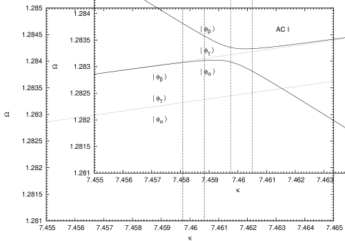
Figure 8: The avoided crossing from Figure 3 (a), now with the relevant odd-parity state included (dotted line). The vertical lines are the $\kappa$ values at which the time-evolution in Figure 9 was obtained.

To analyze the tunneling induced by the Hamiltonian in Eq. (5), we consider again the one-period time-evolution operator $\hat{\rm U}(T)$ defined in Section 3.2 and its eigenvectors, the time-strobed Floquet eigenstates $|\phi_{\alpha}(T)\rangle=|\phi_{\alpha}(0)\rangle$ (we will drop the explicit reference to “time-strobed” in this section). As a particular example, consider the avoided crossing shown in Figure 8 (the same as that shown in Figure 3, but with the odd-parity state now included, shown as a dotted line). At $\kappa=7.456$, a value far from the avoided crossing, the opposite-parity pair of states $|\phi_{\alpha}\rangle$ and $|\phi_{\gamma}\rangle$ are near-degenerate ($|\Omega_{\gamma}-\Omega_{\alpha}|\approx 4.5\times 10^{-6}$) and have localization at $p\approx\pm 5$. The phase space localization of state $|\phi_{\beta}\rangle$ is completely within the central resonance and does not overlap significantly with this pair. We can construct an initial state, localized at either $p\approx 5$ or $-5$, as an equal superposition of the two near-degenerate Floquet states, i.e. $|\psi_{\pm}(0)\rangle=\frac{1}{\sqrt{2}}\left(|\phi_{\alpha}\rangle\pm|\phi_{\gamma}\rangle\right)$. When either is acted on by $\hat{\rm U}(nT)$, the evolution is periodic, oscillating between $p\approx\pm 5$ with a tunneling frequency $\omega_{tun}=|\Omega_{\alpha}-\Omega_{\gamma}|$. The corresponding number of modulation periods for complete oscillation is then $n_{tun}=\omega/\omega_{tun}\approx 5.3\times 10^{6}$.

Figure 9: The evolution of state $|\psi_{+}(0)\rangle$ (created by the superposition of the near-degenerate states at $\kappa=7.456$) under the action of $\hat{\rm U}(T)$ at $\kappa\approx\kappa_{ac}$ (a) and $\kappa=7.4605$ (b).

In the region of the avoided crossing, the odd-parity state $|\phi_{\gamma}\rangle$ will be approximately unchanged, while states $|\phi_{\alpha}\rangle$ and $|\phi_{\beta}\rangle$ become, to lowest order in $\lambda$, superpositions of their unperturbed, Floquet pendulum, counterparts. Therefore, in the neighborhood of the avoided crossing, both $|\phi_{\alpha}\rangle$ and $|\phi_{\beta}\rangle$ will have significant support in the same region of phase space as $|\phi_{\gamma}\rangle$. At the exact position $\kappa_{ac}$ of the avoided crossing, where $|\phi_{\alpha}\rangle$ and $|\phi_{\beta}\rangle$ are an equal superposition of the unperturbed states, the initial conditions localized at either $p\approx 5$ or $-5$ can then be written

$$|\psi_{\pm}(0)\rangle=\frac{1}{2}|\phi_{\alpha}\rangle+\frac{1}{2}|\phi_{\beta}\rangle\pm\frac{1}{\sqrt{2}}|\phi_{\gamma}\rangle\,,$$ (34)

where all three eigenstates are evaluated at $\kappa=\kappa_{ac}$. Applying the time-evolution matrix to $|\psi_{+}(0)\rangle$ we find, after $n$ applications,

$$|\psi_{+}(nT)\rangle =\hat{\rm U}(nT)|\psi_{+}(0)\rangle$$ (35)

$$={\rm e}^{-inT\Omega_{\beta}}\left(\frac{{\rm e}^{-inT\Delta\Omega_{\alpha\beta}}}{2}|\phi_{\alpha}\rangle+\frac{1}{2}|\phi_{\beta}\rangle+\frac{{\rm e}^{-inT\Delta\Omega_{\gamma\beta}}}{\sqrt{2}}|\phi_{\gamma}\rangle\right)\,,$$

where $\Delta\Omega_{ij}\equiv\Omega_{i}-\Omega_{j}$, here. If we make the assumption that $|\Delta\Omega_{\beta\gamma}|=|\Delta\Omega_{\alpha\gamma}|\equiv\Delta$ at $\kappa=\kappa_{ac}$, we see that $|\psi_{+}(\frac{\pi}{\Delta})\rangle\sim|\psi_{-}(0)\rangle$. This three-state process therefore generates a new, larger, tunneling frequency $\omega_{tun}=\Delta$. The time-evolution of $|\psi_{+}(0)\rangle$ at $\kappa\approx\kappa_{ac}$ is shown in Figure 9.a. Notice that the theoretical tunneling period $n_{tun}=\frac{\omega}{\Delta}\approx 1.8\times 10^{5}$ is modulated by a beat period resulting from the small difference $\Delta\Omega_{\beta\gamma}-\Delta\Omega_{\gamma\alpha}$. As the position of the avoided crossing is chosen more precisely, and $\Omega_{\gamma}\rightarrow\frac{\Omega_{\alpha}+\Omega_{\beta}}{2}$, the period of beating goes to infinity.

Between these two extremes of regular two-state and three-state tunneling, at other values of the parameter $\kappa$ along the avoided crossing, the tunneling takes on a beating behavior due to the two eigenvalue differences between the odd-parity state and each even-parity state. An example of this (the evolution of $|\psi_{+}(0)\rangle$ under $\hat{\rm U}(T)$ at $\kappa=7.4605$) is shown in Figure 9.b. For this and all values of the parameter $\kappa$, the evolution of the momentum expectation of $|\psi_{+}(0)\rangle$ is well fit by the simple function

$$\langle p\rangle(nT)=A_{\alpha}\cos\left(\Delta\Omega_{\gamma\alpha}nT\right)+A_{\beta}\cos\left(\Delta\Omega_{\beta\gamma}nT\right)\,,$$ (36)

where $A_{\alpha}$ and $A_{\beta}$ can be related to the overlap of $|\psi_{+}(0)\rangle$ with $|\phi_{\alpha}\rangle$ and $|\phi_{\beta}\rangle$, respectively.

The variation of two-state tunneling frequencies in the vicinity of avoided crossings has been remarked on by many authors [22, 23, 21, 24, 2, 25, 26] in many different systems, and is often attributed to the influence of underlying classical chaos. Classical chaos in a non-perturbative regime will certainly introduce additional complications to the quantum dynamical tunneling process which we have not investigated here (notably the interaction between tunneling through dynamical barriers and free evolution in a region dominated by chaos [27]); and avoided crossings will become larger, more numerous, and may overlap, leading to interaction of more than three relevant states. However, as we have seen in this section, the basic mechanism for “tunneling enhancement” does not necessarily require global chaos but only the non-integrability which leads to avoided crossings. Indeed, for the non-integrability parameter used in this section ($\lambda=5\times 10^{-2}$), the classical phase space has only small regions of chaos.

5.2 Analysis of a Tunneling experiment

As an application of the tunneling results of the previous section, we consider the experiment of Steck, Oskay and Raizen [12]. The Hamiltonian implemented in this atom-optics experiment depends on a single parameter, $\alpha$, and can be considered a special case of that in Eq. (5) by setting $\kappa\approx\alpha/2.17$ (up to a sign difference which can be removed by a $\pi$-translation of the angle variable), $\lambda=\kappa/2$, and $\omega\approx 6.04$. It should be noted that this system is not connected to the Floquet pendulum system since $\lambda$ is not an independent parameter. Instead, in the limit $\lambda,\kappa\rightarrow 0$, the free particle Hamiltonian is obtained.

Figure 10: Floquet eigenvalue curves for the system considered in [12] ($\lambda=\kappa/2$, $\omega\approx 6.04$).

The primary result of the experiments detailed in [12] is the observation of dynamical tunneling, between two resonance islands in the classical phase space (located at $p\approx\pm 3$), which exhibits oscillation frequencies dependent on the parameter value considered and independent of the modulation frequency. In particular, for a range of parameter values, the observed tunneling oscillations were dominated by two primary frequencies. The Floquet eigenvalue curves for the experimental system are shown in Figure 10, and the experimentally observed tunneling frequencies are shown in Figure 11.b, overplotted on the differences of eigenvalues between three particular Floquet eigenstates. These three states exhibit significant localization in the region of the classical resonance islands at some values of the parameter $\kappa$ [11]. The experimental frequencies are well predicted by only two of these differences, namely $\Delta\Omega_{\alpha\gamma}$ and $\Delta\Omega_{\beta\gamma}$.

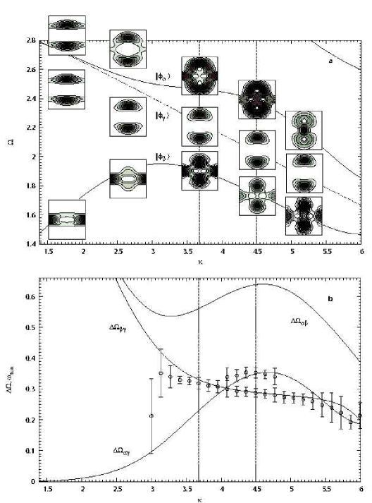
Figure 11: The boxed region of Figure 10 where an avoided crossing occurs between two even parity states (a). The Husimi distributions of these and a third, odd-parity, state are overplotted, with axes of $\theta_{0}\in(0,2\pi)$ and $p\in(-6,6)$. The differences of these three eigenvalues are shown in (c), with experimental tunneling frequencies overplotted (circles, reprinted with permission from Steck, et. al. [12], Fig. 1).

The oscillations seen in the parameter region $\kappa\in[3,4.75]$ are due to the existence of an avoided crossing between the eigenvalues of the even-parity states labelled $|\phi_{\alpha}\rangle$ and $|\phi_{\beta}\rangle$. As can be seen in the overplotted Husimi distributions, these two even-parity states originate at small $\kappa$ values from two disconnected regions of the phase space, the first residing at $p\approx 0$, and the other at the positions of the classical resonance islands where the odd parity state $|\phi_{\gamma}\rangle$ also has its primary support. In passing through this avoided crossing, the odd-parity state retains its original character, while the two even-parity states become mutual superpositions of their small $\kappa$ character. It is clear that this avoided crossing is not of the ideal form considered in the perturbative regime. The superposing effects of this avoided crossing are extend well beyond the minimum eigenvalue separation at $\kappa\approx 3.0$ (see Figure 11.a), due to the natural eigenvalue curvature of a state with the low $\kappa$ character of $|\phi_{\beta}\rangle$ (a simpler example of this is state $(1,0)$ in Figure 2.b). Just past this minimum spacing, the eigenvalue of state $|\phi_{\alpha}\rangle$ curves back downward toward that of $|\phi_{\beta}\rangle$, immediately beginning a second avoided crossing and thus preserving the composite nature of these two even-parity states through $\kappa\approx 6$. As a further complication, in the parameter region $\kappa\in[5,7]$, states $|\phi_{\alpha}\rangle$ and $|\phi_{\beta}\rangle$ are joined by two other even-parity states in a complex and overlapping set of avoided crossings.

Despite these complications, we can identify the dynamical tunneling in the parameter region $\kappa\in[2.5,4.75]$ to be a three-state process involving those states shown in Figure 11.a. As predicted by the results of the previous section, the observed tunneling frequencies involve only differences in Floquet eigenvalue between the odd parity state and the two even parity states. A direct comparison of the oscillations from [12] with the numerically calculated evolution of an initially localized state $|\psi_{+}(0)\rangle$ under $\hat{\rm U}(T)$ is shown in Figure 12 for the values $\kappa=3.68$ and $4.50$. Neglecting dissipation and a momentum offset of the experimental values (due to the fact that not all atoms contributing to the average are participating in the dynamics), there is good agreement in the second case. In the first case, and for all parameter values between $\kappa=3$ and $4$, the experiment seems to pick up only one of the underlying frequencies ($\Delta\Omega_{\gamma\beta}$, while the numerics predict nearly equal contributions from $\Delta\Omega_{\gamma\beta}$ and $\Delta\Omega_{\alpha\gamma}$. It was noted in Reference [28] that the detection of fewer than the predicted number of frequency contributions to the tunneling behavior was also found in another experimental system [10].

Figure 12: Numerical evolution (squares) of a positive momentum centered initial state under the time-evolution operator at $\kappa=3.68$ (a) and $4.50$ (b), with experimental values overplotted (circles, reprinted with permission from Steck, et. al. [12], Fig. 2).

Figure 13: Eigenvalue surfaces, over $\kappa-\lambda$ space, of the even parity Floquet eigenstates involved in the avoided crossing of Figure 11.a. The eigenvalues on the particular curve investigated in reference [12] are overplotted in bold. A dashed line traces the minimum separation of the two surfaces from the diabolical point at $\kappa=0$, $\lambda\approx 2.8$ to the avoided crossing seen in the experiment.

Finally, we would like to consider the origin of the avoided crossing involved in the dynamical tunneling observed in [12]. Figure 13 shows the avoided crossing of Figure 11.a lying on the eigenvalue surfaces $\Omega_{\alpha}$ and $\Omega_{\beta}$ in $\kappa-\lambda$ space. One can see that these two surfaces meet at a diabolical point on the $\kappa=0$ axis, where $\lambda\approx 2.8$. Numerical analysis shows that, in the neighborhood of the diabolical point, the minimum spacing between the two eigenvalue surfaces is linearly dependent on $\kappa$, with

$$\Delta_{\alpha\beta}=9.22\times 10^{-2}\kappa\,.$$ (37)

This result is in good agreement with a perturbation analysis similar to that of Appendix A, but with $\kappa$ as the small expansion parameter. The predicted minimum spacing from such an analysis yields

$$\Delta_{\alpha\beta,{\rm pt}}=2|V^{\prime}_{\alpha\beta}|\kappa\approx 9.2\times 10^{-2}\kappa\,,$$ (38)

where the matrix element must be numerically calculated as the coupling of the two degenerate Floquet eigenstates of the ($\kappa=0.0$,$\lambda=2.8$) system through $\hat{V}^{\prime}=\cos\hat{\theta}$, the coefficient of $\kappa$. Although the avoided crossing in the experiment (Figure 11.a) appears at a parameter value outside the range of validity of perturbation theory, the observed minimum spacing between $\Delta\Omega_{\alpha}$ and $\Delta\Omega_{\beta}$ agrees with Eq. 38 to within a factor of two.

6 Conclusions

We have shown that the minimum spacing of avoided crossings in a near-integrable time-periodic system, and therefore the minimally separated “ridges” of the double-cone structures surrounding a diabolical point, exhibits a power law dependence on the non-integrability parameter, with integer power. A modified degenerate perturbation theory has allowed us to relate the coefficient of this dependence to the direct or indirect coupling of the two related unperturbed Floquet states through the perturbation operator, and the integer power to the number of “photon energies” $\omega$ connecting their related energy eigenvalues. Moreover, the perturbation analysis predicts a qualitatively identical structure for all avoided crossings which allows us to characterize generically their affect on dynamical tunneling. This description was applied to a particular avoided crossing generating multiple-state tunneling oscillations in an experimental system, and its connection to a nearby diabolical point was revealed. It is hoped that these results will provide guidance for the development of new experimental setups which intend to use avoided crossings in the realization of multiple state tunneling processes and adiabatic transitions, or the preparation of Schrödinger’s cat type superposed states.

7 Acknowledgements

The authors thank the Robert A. Welch Foundation (Grant No. F-1051) and the Engineering Research Program of the Office of Basic Energy Sciences at the U.S. Department of Energy (Grant No. DE-FG03-94ER14465) for support of this work. Author LER thanks the Office of Naval Research (Grant No. N00014-03-1-0639) for partial support of this work. The authors also thank Robert Luter for many helpful discussions and Daniel Steck for providing us with the experimental data from reference [12].

Appendix A Perturbation Theory for Avoided Crossings

The Floquet pendulum system $\hat{H}^{0}_{F}(\kappa)$ has a two-fold degeneracy at $\kappa=\kappa_{0}$ where two eigenstates $|\alpha^{0}\rangle\equiv|n_{\alpha}(\kappa_{0}),q_{\alpha}\rangle$ and $|\beta^{0}\rangle\equiv|n_{\beta}(\kappa_{0}),q_{\beta}\rangle$ have eigenvalues $\Omega_{\alpha}(\kappa_{0})=\Omega_{\beta}(\kappa_{0})$. We will use a modified degenerate perturbation theory to lift this degeneracy at the $\kappa$-position of the resulting avoided crossing when $\lambda>0$. In light of the discussion in Section 4.2, we write the Floquet Hamiltonian as

$${\hat{H}}_{F}(\kappa)={\hat{H}}_{F}^{0}+{\delta{\hat{H}}_{F}}\;\Delta\kappa(\lambda)+{\lambda}\;{\hat{V}},$$ (39)

where we now write ${\hat{H}}_{F}^{0}\equiv{\hat{H}}_{F}^{0}(\kappa_{0})$. The operator ${\delta{\hat{H}}_{F}}$ is $\frac{\partial\hat{H}_{F}}{\partial\kappa}=\cos\hat{\theta}$ with the simplifying assumption that this operator is diagonal in the unperturbed basis. This is equivalent to the assumption that the unperturbed eigenvalue curves are linear in the small region of $\kappa$ under consideration. We expand $\Delta\kappa(\lambda)$, setting $\Delta\kappa(0)=0$, so that

$$\Delta\kappa(\lambda)=\Delta\kappa^{(1)}{\lambda}+\Delta\kappa^{(2)}{\lambda}^{2}+\cdots$$ (40)

We expand the near-degenerate eigenstates and eigenvalues in powers of $\lambda$ about their ($\kappa=\kappa_{0},\lambda=0$) values:

$$\begin{split}|\phi{\rangle}&=C_{\alpha}|\alpha^{0}{\rangle}+C_{\beta}|\beta^{0}{\rangle}+{\lambda}|\phi^{1}{\rangle}+{\lambda}^{2}|\phi^{2}{\rangle}+\cdots\\ {\Omega}&={\Omega}^{(0)}+{\lambda}{\Omega}^{(1)}+{\lambda}^{2}{\Omega}^{(2)}+\cdots\end{split}$$ (41)

where $\hat{H}^{0}_{F}|\alpha^{0}\rangle=\Omega^{(0)}|\alpha^{0}\rangle$, $\hat{H}^{0}_{F}|\beta^{0}\rangle=\Omega^{(0)}|\beta^{0}\rangle$ and the zeroth-order eigenstates have been assumed to be a superposition of the two degenerate unperturbed states. As is usual in degenerate perturbation theory, the lowest-order near-degenerate eigenstates and the corrections to their eigenvalues will be the eigenvectors and eigenvalues of a $2\times 2$ matrix in the basis of the two degenerate unperturbed states. At this order, we will make the distinct assignments $|\phi\rangle\rightarrow|\phi_{\pm}\rangle$ (corresponding to the solutions of the quadratic characteristic equation). The final expressions for $C^{\pm}_{\alpha}$, $C^{\pm}_{\beta}$, $|\phi^{i}_{\pm}\rangle$, and $\Omega^{(i>0)}_{\pm}$ will depend on $\kappa$ through the particular choice of the $\Delta\kappa^{(i)}$’s. The Floquet eigenvalue equation (7) for the near-degenerate state now takes the form

$$\left[(\hat{H}_{F}^{0}-{\Omega}^{(0)})~{}\left(C_{\alpha}|\alpha^{0}{\rangle}+C_{\beta}|\beta^{0}{\rangle}\right)\right]\\ +\lambda\left[(\hat{H}_{F}^{0}-{\Omega}^{(0)})|{\phi^{1}}{\rangle}+\left(\Delta\kappa^{(1)}{\delta{\hat{H}}_{F}}+\hat{V}-{\Omega}^{(1)}\right)~{}\left(C_{\alpha}|\alpha^{0}{\rangle}+C_{\beta}|\beta^{0}{\rangle}\right)\right]\\ +\lambda^{2}\left[(\hat{H}_{F}^{0}-{\Omega}^{(0)})|{\phi^{2}}{\rangle}+(\Delta\kappa^{(1)}{\delta{\hat{H}}_{F}}+\hat{V}-{\Omega}^{(1)})|{\phi^{1}}{\rangle}\right.\\ \left.+(\Delta\kappa^{(2)}{\delta{\hat{H}}_{F}}-{\Omega}^{(2)})~{}(C_{\alpha}|\alpha^{0}{\rangle}+C_{\beta}|\beta^{0}{\rangle})\right]+\cdots=0\,.$$ (42)

A.1 First-order results

At first order in $\lambda$ we have the eigenvalue equation

$$(\hat{H}_{F}^{0}-{\Omega}^{(0)})|{\phi^{1}}{\rangle}+(\Delta\kappa^{(1)}{\delta{\hat{H}}_{F}}+\hat{V}-{\Omega}^{(1)})(C_{\alpha}|\alpha^{0}{\rangle}+C_{\beta}|\beta^{0}{\rangle})=0\,.$$ (43)

If we now act on this equation with ${\langle}\alpha^{0}|$ and then with ${\langle}\beta^{0}|$, we obtain

$$\left(\begin{array}[]{cc}\Delta\kappa^{(1)}{\delta}E_{\alpha}+V_{\alpha\alpha}-{\Omega}^{(1)}&V_{\alpha\beta}\\ V_{\beta\alpha}&\Delta\kappa^{(1)}{\delta}E_{\beta}+V_{\beta\beta}-{\Omega}^{(1)}\\ \end{array}\right)\left(\begin{array}[]{c}C_{\alpha}\\ C_{\beta}\\ \end{array}\right)={\bf 0}\,.$$ (44)

where $V_{ij}$ are the matrix elements of the perturbation in the basis of the degenerate unperturbed eigenstates,

$$\delta E_{i}\equiv\langle\langle n_{i},q_{i}|\delta\hat{H}_{F}|n_{i},q_{i}\rangle\rangle=\langle n_{i}|\cos\hat{\theta}|n_{i}\rangle\,,$$ (45)

and we have used the identity

$$1=\sum_{\gamma}|\gamma^{0}\rangle\langle\gamma^{0}|\equiv\sum_{\left(n_{\gamma},q_{\gamma}\right)}|n_{\gamma},q_{\gamma}\rangle\langle n_{\gamma},q_{\gamma}|=\sum_{n,q=-\infty}^{\infty}|n,q\rangle\langle n,q|\,.$$ (46)

At this point, we must consider two possible cases: $V_{\alpha\beta}\neq 0$ and $V_{\alpha\beta}=0$. In the first case, a nontrivial solution for the $C_{i}$ requires first-order corrections to the unperturbed Floquet eigenvalues

$${\Omega}^{(1)}_{\pm}=\frac{1}{2}\left[V_{\alpha\alpha}+V_{\beta\beta}+\Delta\kappa^{(1)}({\delta}E_{\alpha}+{\delta}E_{\beta})\right]\\ \pm\frac{1}{2}\left\{\left[(V_{\alpha\alpha}-V_{\beta\beta})+\Delta\kappa^{(1)}({\delta}E_{\alpha}-{\delta}E_{\beta})\right]^{2}+4|V_{\alpha\beta}|^{2}\right\}^{\frac{1}{2}}\,.$$ (47)

We can then write the spacing between the two Floquet eigenvalues

$$\Delta{\Omega}{\equiv}{\Omega}^{(1)}_{+}-{\Omega}^{(1)}_{-}=\lambda\left\{\left[(V_{\alpha\alpha}-V_{\beta\beta})+\Delta\kappa^{(1)}({\delta}E_{\alpha}-{\delta}E_{\beta})\right]^{2}+4|V_{\alpha\beta}|^{2}\right\}^{\frac{1}{2}}+O(\lambda^{2})\,.$$ (48)

In order to determine the particular value of $\Delta\kappa^{(1)}$ at which the minimum spacing occurs, we solve the extremal equation

$$\left(\frac{\partial\Delta\Omega}{\partial\Delta\kappa}\right)_{\lambda}=\frac{1}{\lambda}\left(\frac{\partial\Delta\Omega}{\partial\Delta\kappa^{(1)}}\right)_{\lambda,\Delta\kappa^{(m)}}=0\quad(m\neq 1)\,,$$ (49)

finding that

$$\Delta\kappa^{(1)}_{ac}=\frac{V_{\beta\beta}-V_{\alpha\alpha}}{{\delta}E_{\alpha}-{\delta}E_{\beta}}\,.$$ (50)

If we substitute this into Eq. (47), we obtain first order corrections to the eigenvalues of

$$\Omega^{(1)}_{\pm}=\frac{V_{\beta\beta}\delta E_{\alpha}-V_{\alpha\alpha}\delta E_{\beta}}{\delta E_{\alpha}-\delta E_{\beta}}\pm|V_{\alpha\beta}|\,.$$ (51)

Therefore, we find the minimum splitting to be

$$\Delta_{\alpha\beta}=2\lambda|V_{\alpha\beta}|+O(\lambda^{2})\,.$$ (52)

In the second case ($V_{\alpha\beta}=0$), we find that the nearest approach of the two Floquet eigenvalues is in fact a crossing (to first order in $\lambda$). In this case we define $\Delta\kappa^{(1)}_{ac}$ to be the offset of this crossing, i.e.

$${\Delta}{\Omega}=O(\lambda^{2})~{}~{}~{}{\rm at}~{}~{}~{}\Delta\kappa^{(1)}_{ac}\equiv\frac{V_{\beta\beta}-V_{\alpha\alpha}}{{\delta}E_{\alpha}-{\delta}E_{\beta}}.$$ (53)

The coefficients $C_{i}$ remain undetermined until the degeneracy is broken.

A.2 Second-order results ($V_{\alpha\beta}=0$)

For the case $V_{\alpha\beta}=0$, the zeroth order states must be determined from the second order equation, which takes the form

$$(\hat{H}_{F}^{0}-{\Omega}^{(0)})|{\phi^{2}}{\rangle}+(\Delta\kappa^{(1)}{\delta{\hat{H}}_{F}}+\hat{V}-{\Omega}^{(1)})|{\phi^{1}}{\rangle}$$

$$+(\Delta\kappa^{(2)}{\delta{\hat{H}}_{F}}-{\Omega}^{(2)})~{}(C_{\alpha}|\alpha^{0}{\rangle}+C_{\beta}|\beta^{0}{\rangle})=0\,,$$ (54)

Following the same procedure as in first order, we obtain

$$\left(\begin{array}[]{cc}\Delta\kappa^{(2)}{\delta}E_{\alpha}+{v}_{\alpha\alpha}-{\Omega}^{(2)}&{v}_{\alpha\beta}\\ {v}_{\beta\alpha}&\Delta\kappa^{(2)}{\delta}E_{\beta}+{v}_{\beta\beta}-{\Omega}^{(2)}\\ \end{array}\right)\left(\begin{array}[]{c}C_{\alpha}\\ C_{\beta}\\ \end{array}\right)={\bf 0}\,,$$ (55)

where we have used the first-order result

$$\langle\gamma^{0}|\phi^{1}\rangle=\frac{V_{\gamma\alpha}C_{\alpha}+V_{\gamma\beta}C_{\beta}}{\Omega^{(0)}-\Omega^{(0)}_{\gamma}}\quad\left(\gamma\not\in\{\alpha,\beta\}\right)$$ (56)

with $\Omega^{(0)}_{\gamma}=\langle n_{\gamma},q_{\gamma}|\hat{H}_{F}^{0}|n_{\gamma},q_{\gamma}\rangle$, and where we have defined

$${v}_{ij}\equiv\sum_{\gamma\not\in\{\alpha,\beta\}}\frac{V_{i\gamma}V_{\gamma j}}{\Omega^{(0)}-{\Omega}^{(0)}_{\gamma}}\quad\left(i,j\in\{\alpha,\beta\}\right)\,.$$ (57)

Again we must consider two cases: ${v}_{\alpha\beta}\neq 0$ and ${v}_{\alpha\beta}=0$. In the first case, our procedure for determining $\Delta\kappa^{(2)}_{ac}$ is identical to that of first-order and we obtain

$$\Delta\kappa^{(2)}_{ac}=\frac{{v}_{\beta\beta}-{v}_{\alpha\alpha}}{{\delta}E_{\alpha}-{\delta}E_{\beta}}\quad{\rm and}\quad\Delta_{\alpha\beta}=2\lambda^{2}|{v}_{\alpha\beta}|+O(\lambda^{3})\,.$$ (58)

In the case that $v_{\alpha\beta}=0$, we find that ${\Delta}{\Omega}=O(\lambda^{3})$ at an offset of

$$\Delta\kappa^{(2)}_{ac}=\frac{{v}_{\beta\beta}-{v}_{\alpha\alpha}}{{\delta}E_{\alpha}-{\delta}E_{\beta}}\,.$$ (59)

A.3 Third-order results ($V_{\alpha\beta}=0$ and $v_{\alpha\beta}=0$)

If the conditions $V_{\alpha\beta}=0$ and $v_{\alpha\beta}=0$ are satisfied, we can attempt to lift the degeneracy at order $\lambda^{3}$. We obtain the following results

$$\left(\begin{array}[]{cc}\Delta\kappa^{(3)}{\delta}E_{\alpha}+\mathfrak{v}_{\alpha\alpha}+\bar{\mathfrak{v}}_{\alpha}-{\Omega}^{(3)}&\mathfrak{v}_{\alpha\beta}\\ \mathfrak{v}_{\beta\alpha}&\Delta\kappa^{(3)}{\delta}E_{\beta}+\mathfrak{v}_{\beta\beta}+\bar{\mathfrak{v}}_{\beta}-{\Omega}^{(3)}\\ \end{array}\right)\left(\begin{array}[]{c}C_{\alpha}\\ C_{\beta}\\ \end{array}\right)={\bf 0}\,,$$ (60)

where we have defined

$$\mathfrak{v}_{ij}\equiv\sum_{\gamma,\sigma\not\in\{\alpha,\beta\}}\frac{V_{i\gamma}V_{\gamma\sigma}V_{\sigma j}}{\left(\Omega^{(0)}-{\Omega}^{(0)}_{\gamma}\right)\left(\Omega^{(0)}-\Omega^{(0)}_{\sigma}\right)}\quad\left(i,j\in\{\alpha,\beta\}\right)\,,$$ (61)

and

$$\bar{\mathfrak{v}}_{i}\equiv\sum_{\gamma\not\in\{\alpha,\beta\}}\frac{\left(\Delta\kappa^{(1)}\delta E_{\gamma}-\Omega^{(1)}\right)V_{i\gamma}V_{\gamma i}}{\left(\Omega^{(0)}-{\Omega}^{(0)}_{\gamma}\right)^{2}}\quad\left(i\in\{\alpha,\beta\}\right)\,,$$ (62)

and where we have used an expression for $\langle\gamma^{0}|\phi^{2}\rangle$ (analogous to Equation 56) determined from the second-order equation.

These equations are nearly of the same form as those at first and second order. By the same procedure we determine

$$\Delta\kappa^{(3)}_{ac}=\frac{\mathfrak{v}_{\beta\beta}+\bar{\mathfrak{v}}_{\beta}-\mathfrak{v}_{\alpha\alpha}-\bar{\mathfrak{v}}_{\alpha}}{{\delta}E_{\alpha}-{\delta}E_{\beta}}\quad{\rm and}\quad\Delta_{\alpha\beta}=2\lambda^{3}|\mathfrak{v}_{\alpha\beta}|+O(\lambda^{4})\,,$$ (63)

for the case that $\mathfrak{v}_{\alpha\beta}\neq 0$ and $\Delta_{\alpha\beta}=O(\lambda^{4})$ when $\mathfrak{v}_{\alpha\beta}=0$.

References

• [1] J. von Neumann and E. Wigner, Physik. Zeitschr. 30, 465 (1929). English translation in: R.S. Knox and A. Gold, Symmetry in the solid state (W.A. Benjamin, New York, 1964).
• [2] S. Tomsovic and D. Ullmo, Phys. Rev. E 50, 145 (1994).
• [3] K. Na and L.E. Reichl, Phys. Rev. A 70, 063405 (2004).
• [4] T. Timberlake and L. E. Reichl, Phys. Rev. A 59, 2886 (1999).
• [5] L.E. Reichl, Transistion to Chaos in Conservative Classical Systems: Quantum Manifestations (Springer-Verlag, New York, 1992).
• [6] M.V. Berry and M. Wilkinson, Proc. Roy. Soc. Lond. A392, 15 (1984).
• [7] R. Graham, M. Schlautmann, and P. Zoller, Phys. Rev. A 45, R19 (1992).
• [8] F.L. Moore, J.C. Robinson, C. Bharucha, P.E. Williams, and M.G. Raizen, Phys. Rev. Lett. 73, 2974 (1994).
• [9] D.A. Steck, W.H. Oskay, and M.G. Raizen, Science 293, 274 (2001).
• [10] W.K. Hensinger, H. Häffner, A. Browaeys, N.R. Heckenberg, K. Helmerson, C. McKenzie, G.J. Milburn, W.D. Phillips, S.L. Rolston, H. Rubinsztein-Dunlop, and B. Upcroft, Nature 412, 52 (2001).
• [11] R. Luter and L.E. Reichl, Phys. Rev. E 66, 053615 (2002).
• [12] D.A. Steck, W.H. Oskay, and M.G. Raizen. Phys. Rev. Lett. 88, 120406 (2002).
• [13] M. Abramowitz and I.A. Stegun, Handbook of Mathematical Functions, Applied Mathematics Series no. 55 (U.S. Dept. of Commerce, Washington D.C., 1972).
• [14] H. Sambe, Phys. Rev. A 7, 2203 (1973).
• [15] A. Ya. Dzyublik, Theoretical and Mathematical Physics 87, 393 (1991).
• [16] K. Husimi, Proc. Phys. Math. Soc. Japan 22, 264 (1940).
• [17] A. Knauf and Y.G. Sinai, Classical Nonintegrability, Quantum Chaos, DMV Seminar Band 27 (Birkhäuser Verlag, Basel, 1997).
• [18] W.D. Heiss and A.L. Sannino, J. Phys. A: Math Gen. 23, 1167 (1990).
• [19] M.J. Davis and E.J. Heller, J. Chem. Phys. 75, 246 (1981).
• [20] J.J. Sakurai, Modern Quantum Mechanics (Addison-Wesley Pub., Reading MA, 1994).
• [21] F. Grossmann, T. Dittrich, P. Jung, and P. Hänggi, Phys. Rev. A 67, 516 (1991).
• [22] M. Latka, P. Grigolini, and B.J. West, Phys. Rev. A 50, 1071 (1994).
• [23] M. Latka, P. Grigolini, and B.J. West, Phys. Rev. A 50, 596 (1994).
• [24] I. Vorobeichik and N. Moiseyev, Phys. Rev. A 59, 2511 (1999).
• [25] O. Brodier, P. Schlagheck, and D. Ullmo, Phys. Rev. Lett. 87, 064101 (2001).
• [26] A. Mouchet and D. Delande, Phys. Rev. E 67, 046216 (2003).
• [27] V.I. Podolskiy and E.E. Narimanov, Phys. Rev. Lett. 91, 263601 (2003).
• [28] R. Luter and L.E. Reichl, J. Phys. Soc. Jpn. 72, Suppl. C, 134 (2003).