Exact exchange optimized effective potential and self-compression of
stabilized jellium clusters

Abstract

In this work, we have used the exchange-only optimized effective potential in the self-consistent calculations of the density functional Kohn-Sham equations for simple metal clusters in stabilized jellium model with self-compression. The results for the closed-shell clusters of Al, Li, Na, K, and Cs with $N=$2, 8, 18, 20, 34, and 40 show that the clusters are $3\%$ more compressed here than in the local spin density approximation. On the other hand, in the LSDA, neglecting the correlation results in a contraction by $1.4\%$.

I Introduction

The Kohn-Sham (KS)KS65 density functional theory (DFT)HK64 is one of the most powerful techniques in electronic structure calculations. However, the exact form of the exchange-correlation functional is still unknown and, in practice, one must use approximations. The accuracy of the predictions of the properties depends on how one approximates this functional. The simplest one is the local spin density approximation (LSDA) in which one uses the properties of the uniform electron gas locally KS65 . This approximation is in principle appropriate for systems in which the variations of the spin densities $n_{\sigma}$ are sufficiently slow. For finite systems and surfaces which are highly inhomogeneous, the generalized gradient approximation (GGA)Perdew96 is more appropriate. In spite of the success of the LSDA and GGA, it is observed that in some cases these approximations fail to predict even qualitatively correct behaviorsSchmid ; Varga ; Leung ; Dufek . On the other hand, appropriate self-interaction corrected versions of these approximations are observed to lead to correct behaviorsDufek ; Engel93 . These observations motivates one to use functionals in which the self-interaction contribution is removed exactly. One of the functionals, which satisfies this constraint, is the exact exchange (EEX) orbital dependent functional. Using the EEX functional leads to the correct asymptotic behavior of the KS potential as well as to correct results for the high density limit in which the exchange energy is dominated Perdew01 . Although neglecting the correlation effects in orbital dependent functionals fails to reproduce the dispersion forces such as the van der Waals forcesEngel99 ; Magyar04 , the EEX in some respects is advantageous over the local and semi-local approximationsMagyar04 ; Kummel04 . To obtain the local exchange potential from the orbital dependent functional, one should solve the optimized effective potential (OEP) integral equation. Recently, Kümmel and Perdew KummelPRL03 ; KummelPRB03 have invented an iterative method which allows one to solve the OEP integral equation accurately and efficiently even for three dimensional systems. This method is used in this work.

To simplify the cluster problem, one notes that the properties of alkali metals are dominantly determined by the delocalized valence electrons. In these metals, the Fermi wavelengths of the valence electrons are much larger than the metal lattice constants and the pseudo-potentials of the ions do not significantly affect the electronic structure. This fact allows one to replace the discrete ionic structure by a homogeneous positive charge background which is called jellium model (JM). In its simplest form, one applies the JM to metal clusters by replacing the ions of an $N$-atom cluster with a sphere of uniform positive charge density and radius $R=(zN)^{1/3}r_{s}$, where $z$ is the valence of the atom and $r_{s}$ is the bulk value of the Wigner-Seitz (WS) radius for valence electronsPayami99 ; Payami01 ; Payami-PSS04 . Assuming the spherical geometry is justified only for closed-shell clusters which is the subject in this work. However, it is a known fact that the JM has some drawbacksLang70 ; Ashcroft67 . The stabilized jellium model (SJM) in its original formPerdew90 was the first attempt to overcome the deficiencies of the JM and still keeping the simplicity of the JM. Application of the SJM to simple metals and metal clusters has shown significant improvements over the JM resultsPerdew90 . However, for small metal clusters the surface effects are important and the cluster is self-compressed due to its surface tension. This effect has been successfully taken into account by the SJM which is called SJM with self-compression (SJM-SC)Perdew93 ; Payami-CJ04 . Application of the LSDA-SJM-SC to neutral metal clusters has shown that the equilibrium $r_{s}$ values of small clusters are smaller than their bulk counterparts and approaches to it for very large clusters. This trend is consistent with the results of ab. initio. calculationsRothlisberger ; Payami-PSS01 .

In this work we have used the EEX-SJM-SC to obtain the equilibrium sizes and energies of closed-shell neutral $N$-electron clusters of Al, Li, Na, K, and Cs for $N$=2, 8, 18, 20, 34, and 40 (for Al, $N$ = 18 corresponds to Al₆ cluster and other values do not correspond to a real Al_n). In order to have an estimate for the self-interaction effects, we have repeated the calculations for exchange-only local spin density approximation (x-LSDA) in which the spin-polarized version of the Dirac form, $E_{x}=c_{x}\int d{{\bf r}}\;n^{4/3}$, is used. Comparison of the results shows that (except for $N=40$ in Al case) the relation $\bar{r}_{EEX}<\bar{r}_{x-LSDA}<\bar{r}_{LSDA}$. The organization of this paper is as follows. In section II we explain the calculational schemes. Section III is devoted to the results of our calculations and finally, we conclude this work in section IV.

II Calculational schemes

In this section we first explain how to implement the exact exchange in the SJM, and then will explain the procedure for the OEP calculations.

II.1 Exact exchange stabilized jellium model

As in the original SJMPerdew90 , here the Ashcroft empty core pseudo-potentialAshcroft66 is used for the interaction of an ion of charge $z$ with an electron at a relative distance $r$:

$$w(r)=\left\{\begin{array}[]{ccc}-2z/r&,&(r>r_{c})\\ 0&,&(r<r_{c})\end{array}\right.$$ (1)

The core radius, $r_{c}$, will be fixed by setting the pressure of the bulk system equal to zero. In the EEX-SJM, the average energy per valence electron in the bulk with density $n$ is given by

$$\varepsilon(n)=t_{s}(n)+\varepsilon_{x}(n)+\bar{w}_{R}(n,r_{c})+\varepsilon_{M}(n),$$ (2)

with

$$t_{s}(n)=c_{k}n^{2/3},$$ (3)

$$\varepsilon_{x}(n)=c_{x}n^{1/3},$$ (4)

$$c_{k}=\frac{3}{5}(3\pi^{2})^{2/3},\;\;\;\;\;\;c_{x}=\frac{3}{2}(3/\pi)^{1/3}.$$ (5)

All equations throughout this paper are expressed in Rydberg atomic units. Here $t_{s}$ and $\varepsilon_{x}$ are the kinetic and exchange energy per particle, respectively. $\bar{w}_{R}$ is the average value of the repulsive part of the pseudo-potential ($\bar{w}_{R}=4\pi nr_{c}^{2}$), and $\varepsilon_{M}$ is the average Madelung energy. Demanding zero pressure for the bulk system at equilibrium yields:

$$\left\{2t_{s}(n)+\varepsilon_{x}(n)+12\pi nr_{c}^{2}+\varepsilon_{M}(n)\right\}_{n=n^{B}}=0.$$ (6)

Solution of this equation for $r_{c}$ gives

$$r_{c}(r_{s}^{B})=\frac{(r_{s}^{B})^{3/2}}{3}\left\{-2t_{s}(r_{s})-\varepsilon_{x}(r_{s})-\varepsilon_{M}(r_{s})\right\}_{r_{s}=r_{s}^{B}}^{1/2}.$$ (7)

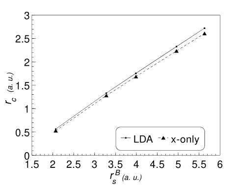
Figure 1: Pseudo-potential core radii in atomic units for different $r_{s}^{B}$ values.

In Fig. 1 we have plotted the core radii for different values of $r_{s}^{B}$ which assume 2.07, 3.28, 3.99, 4.96, and 5.63 for Al, Li, Na, K, and Cs, respectively. The result is compared with the case in which the correlation energy is also incorporated (see Eq.(26) of Ref.Perdew90 ). As is seen, to stabilize the bulk system in the EEX case, the core radii assume smaller values.

As in the original SJMPerdew90 (but in the absence of the correlation energy component), at equilibrium density we have

$$\langle\delta v\rangle_{WS}=-\frac{1}{3}[2t_{s}(n^{B})+\varepsilon_{x}(n^{B})].$$ (8)

Here, $\langle\delta v\rangle_{WS}$ is the average of the difference potential over the WS cell and the difference potential, $\delta v$, is defined as the difference between the pseudo-potential of a lattice of ions and the electrostatic potential of the jellium positive background. Once the values of $\langle\delta v\rangle_{WS}$ and $r_{c}$ as functions of $r_{s}^{B}$ are found, the EEX-SJM total energy of a cluster becomes

$$E_{EEX-SJM}[n_{\uparrow},n_{\downarrow},r_{s},r_{s}^{B}]=E_{EEX-JM}[n_{\uparrow},n_{\downarrow},r_{s}]$$

$$+(\varepsilon_{M}+\bar{w}_{R})\int d{{\bf r}}\;n_{+}({{\bf r}})\;\;\;\;\;$$

$$+\langle\delta v\rangle_{WS}\int d{{\bf r}}\;\Theta({{\bf r}})[n({{\bf r}})-n_{+}({{\bf r}})].$$ (9)

Here,

$$E_{EEX-JM}[n_{\uparrow},n_{\downarrow},r_{s}]=T_{s}[n_{\uparrow},n_{\downarrow}]+E_{x}[n_{\uparrow},n_{\downarrow}]$$

$$+\frac{1}{2}\int d{{\bf r}}\;\phi([n,n_{+}];{{\bf r}})\,[n({{\bf r}})-n_{+}({{\bf r}})],$$ (10)

$$E_{x}=\sum_{\sigma=\uparrow,\downarrow}\sum_{i,j=1}^{N_{\sigma}}\int d{{\bf r}}\,d{{\bf r}^{\prime}}\frac{\phi_{i\sigma}^{*}({{\bf r}})\phi_{j\sigma}^{*}({{\bf r}^{\prime}})\phi_{j\sigma}({{\bf r}})\phi_{i\sigma}({{\bf r}^{\prime}})}{\mid{{\bf r}}-{{\bf r}^{\prime}}\mid},$$ (11)

$$\phi([n,n_{+}];{{\bf r}})=2\int d{{\bf r}^{\prime}}\frac{[n({{\bf r}^{\prime}})-n_{+}({{\bf r}^{\prime}})]}{\mid{{\bf r}}-{{\bf r}^{\prime}}\mid},$$ (12)

$$n({{\bf r}})=\sum_{\sigma=\uparrow,\downarrow}\sum_{i=1}^{N_{\sigma}}\mid\phi_{i\sigma}({{\bf r}})\mid^{2},$$ (13)

$$n_{+}({{\bf r}})=n\theta(R-r);\;\;\;\;\;\;n=\frac{3}{4\pi r_{s}^{3}}.$$ (14)

To obtain the equilibrium size and energy of an $N$-atom cluster in EEX-SJM-SC, we solve the equation

$$\left.\frac{\partial}{\partial r_{s}}E(N,r_{s},r_{c})\right|_{r_{s}=\bar{r}_{s}(N)}=0,$$ (15)

where $N$ and $r_{c}$ are kept constant and $E$ is given by Eq. (II.1). The preocedure for the x-LSDA is the same as above except for that the Dirac exchange energy must be used.

II.2 The OEP equations

Kümmel and PerdewKummelPRB03 have proved, in a simple way, that the OEP integral equation is equivalent to

$$\sum_{i=1}^{N_{\sigma}}\psi_{i\sigma}^{*}({{\bf r}})\phi_{i\sigma}({{\bf r}})+c.c.=0.$$ (16)

$\phi_{i\sigma}$ are the self-consistent KS orbitals and $\psi_{i\sigma}$ are orbital shifts. The self-consistent orbital shifts and the local exchange potentials are obtained from the iterative solutions of inhomogeneous KS equations. Taking spherical geometry for the jellium background and inserting

$$\phi_{i\sigma}({{\bf r}})=\frac{\chi_{i\sigma}(r)}{r}Y_{l_{i},m_{i}}(\Omega),$$ (17)

and

$$\psi_{i\sigma}({{\bf r}})=\frac{\xi_{i\sigma}(r)}{r}Y_{l_{i},m_{i}}(\Omega),$$ (18)

in to the inhomogeneous KS equation (Eq.(21) of Ref.KummelPRB03 ) one obtainsPayami05

$$\left[\frac{d^{2}}{dr^{2}}+\varepsilon_{i\sigma}-v_{eff\sigma}(r)-\frac{l_{i}(l_{i}+1)}{r^{2}}\right]\xi_{i\sigma}(r)=q_{i\sigma}(r).$$ (19)

Here, $\varepsilon_{i\sigma}$ are the KS eigenvalues and

$$v_{eff\sigma}({{\bf r}})=v({{\bf r}})+v_{H}({{\bf r}})+v_{x\sigma}({{\bf r}}),$$ (20)

$$v_{H}({{\bf r}})=2\int d{{\bf r}}\,\frac{n({{\bf r}^{\prime}})}{\mid{{\bf r}}-{{\bf r}^{\prime}}\mid}.$$ (21)

The right hand side of Eq. (19) can be written as

$$q_{i\sigma}(r)=q_{i\sigma}^{(1)}(r)+q_{i\sigma}^{(2)}(r),$$ (22)

with

$$q_{i\sigma}^{(1)}(r)=\left[v_{xc\sigma}(r)-\bar{v}_{xci\sigma}+\bar{u}_{xci\sigma}\right]\chi_{i\sigma}(r),$$ (23)

and

$$q_{i\sigma}^{(2)}(r)=2\sum_{j=1}^{N_{\sigma}}\sum_{l=|l_{i}-l_{j}|}^{l_{i}+l_{j}}\frac{4\pi}{2l+1}\chi_{j\sigma}(r)B_{\sigma}(i,j,l;r)$$

$$\times\overline{\left[I(l_{j}m_{j},l_{i}m_{i},lm_{j}-m_{i})\right]^{2}}.$$ (24)

The quantities $B$ and $I$ in Eq. (II.2) are defined as

$$B_{\sigma}(i,j,l;r)=\int_{r^{\prime}=0}^{r}dr^{\prime}\chi_{i\sigma}(r^{\prime})\chi_{j\sigma}(r^{\prime})\frac{{r^{\prime}}^{l}}{r^{l+1}}$$

$$+\int_{r^{\prime}=r}^{\infty}dr^{\prime}\chi_{i\sigma}(r^{\prime})\chi_{j\sigma}(r^{\prime})\frac{r^{l}}{{r^{\prime}}^{l+1}}$$ (25)

$$I(l_{j}m_{j},l_{i}m_{i},lm)=\int d\Omega\;Y_{l_{j}m_{j}}^{*}(\Omega)Y_{l_{i}m_{i}}(\Omega)Y_{lm}(\Omega),$$ (26)

and the bar over $I^{2}$ implies average over $m_{i}$ and $m_{j}$. Also, the expression for $\bar{u}_{xi\sigma}$ reduces to

$$\bar{u}_{xi\sigma}=-2\sum_{j=1}^{N_{\sigma}}\sum_{l=|l_{i}-l_{j}|}^{l_{i}+l_{j}}\frac{4\pi}{2l+1}\overline{\left[I(l_{j}m_{j},l_{i}m_{i},lm_{j}-m_{i})\right]^{2}}$$

$$\times\int_{0}^{\infty}dr\;\chi_{i\sigma}(r)\chi_{j\sigma}(r)B_{\sigma}(i,j,l;r).\;\;\;$$ (27)

The procedure for the self-consistent iterative solutions of the OEP equations is explained in Refs.KummelPRB03 ; Payami05 .

In Fig. 2, the self-consistent source terms $q_{i\sigma}(r)$ of Eq. (19) are plotted for the equilibrium size of Na₁₈ cluster. The corresponding orbital shifts $\xi_{i\sigma}(r)$ are shown in Fig.3.

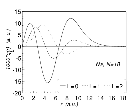
Figure 2: Right hand side of Eq. (19) for the self-consistent equilibrium size of Na₁₈.

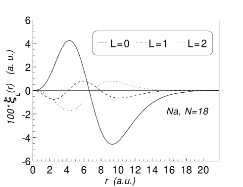
Figure 3: Orbital shifts in atomic units for the self-consistent equilibrium size of Na₁₈.

III Results and discussion

We have used the EEX-SJM-SC to obtain the equilibrium sizes and energies of closed-shell 2, 8, 18, 20, 34, and 40-electron neutral clusters of Al, Li, Na, K, and Cs.

In Table 1 we have listed the equilibrium $r_{s}$ values, total energies and exchange energies. As is seen, the equilibrium $r_{s}$ values of the clusters are almost the same up to 3 decimals for the KLI and OEP schemes whereas, there are significant differences between the OEP, x-LSDA, and LSDA values. As an example, we have plotted the equilibrium $r_{s}$ values of the closed-shell K_N clusters in Fig. 4. It shows that the LSDA predicts larger cluster sizes than the x-LSDA and OEP.

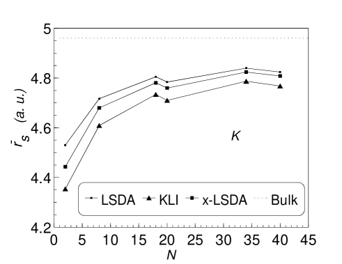
Figure 4: Equilibrium $r_{s}$ values of K_N clusters for different sizes. The dotted line is $r_{s}^{B}$. KLI and OEP predict smaller sizes for the clusters than the x-LSDA and LSDA.

To illustrate the trend in the $\bar{r}_{s}$ values, we plot the difference $(\bar{r}_{s}^{\rm LSD}-\bar{r}_{s}^{\rm KLI})$ for all species in Fig. 5. One notes that for a given element, the difference is larger for smaller clusters. On the other hand, the difference for the lower-density element is higher. However, the difference is about $3\%$ on average. We therefore conclude that the EEX-SJM-SC predicts smaller bond lengths compared to the LSDA-SJM-SC. Comparison of the $\bar{r}_{s}$ values for the LSDA and x-LSDA shows that bond lengths in the LSDA is about $1.4\%$ larger on average. This difference should be attributed to the correlation effects. On the other hand, the same comparison between x-LSDA and KLI shows that, except for $N=40$ in Al, $\bar{r}_{x-LSDA}>\bar{r}_{KLI}$ by $1.5\%$ on average. This difference is due to the self-interaction effects in the Dirac form for the exchange functional.

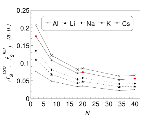
Figure 5: Difference in the equilibrium $r_{s}$ values of clusters with different sizes. The difference is larger for lower-density elements.

Comparison of the equilibrium total energies of the OEP and KLI shows that OEP energies are on average $0.02\%$ more negative. This result should be compared to the simple JM resultsPayami05 which is $1.2\%$. On the other hand, comparison of the exchange energies shows that on the average, the exchange energies in OEP is $0.34\%$ more negative than those in the KLI.

In Table 2, we have listed the lowest and highest occupied KS eigenvalues for different schemes. As in the simple JM Payami05 , the OEP KS eigenvalue bands are contracted relative to those of the KLI. That is, for all $N$, the relation $\Delta^{\rm OEP}<\Delta^{KLI}$ holds. Here, $\Delta=\varepsilon_{H}-\varepsilon_{L}$ is the difference between the maximum occupied and minimum occupied KS eigenvalues. For the same external potential, the OEP and KLI results coincide for two-electron systems and $\Delta=0$. The results in Table2 show that the maximum relative contraction, $|\Delta^{\rm OEP}-\Delta^{KLI}|/\Delta^{KLI}$, is 2.7$\%$ which corresponds to Cs₁₈.

The same comparisons between OEP and x-LSDA shows that $E^{OEP}<E^{x-LSDA}$ by $5.2\%$ on average, and $E_{x}^{OEP}<E_{x}^{x-LSDA}$ by $11\%$ on average. The band widths do not show any regular pattern, however, in the OEP the bands mostly contract relative to the x-LSDA.

Finally, we compare the results of LSDA and x-LSDA, which will show the correlation effects. As is seen in Table 1, the total energies are close to each other for the high-density cases. That is, in the high density limit the exchange dominates the correlation. However, the total energies in the LSDA are more negative by $10\%$ on average which is due to the correlation effects. On the other hand, the difference in the exchange energies is about $0.96\%$ on average which is quite a small fraction. In the high density limit, the inequality $E_{x}^{x-LSD}<E_{x}^{LSDA}$ holds whereas, in the low density limit the inequality changes sign.

Table 1: Equilibrium sizes, $\bar{r}_{s}$, in bohrs, the absolute values of total and exchange energies in rydbergs are compared for KLI, OEP,x-LSDA, and LSDA schemes. In the LSDA, the total energies include the correlation energies as well.

			KLI			OEP			x-LSDA			LSDA
Atom	$r_{s}^{B}$	$N$	$\bar{r}_{s}$	$-\bar{E}$	$-E_{x}$	$\bar{r}_{s}$	$-\bar{E}$	$-E_{x}$	$\bar{r}_{s}$	$-\bar{E}$	$-E_{x}$	$\bar{r}_{s}$	$-\bar{E}$	$-E_{x}$
Al	2.07	2	1.430	1.5700	0.9253	1.430	1.5700	0.9253	1.468	1.4364	0.7574	1.506	1.5585	0.7541
		8	1.744	5.8640	3.6018	1.744	5.8647	3.6089	1.775	5.5768	3.2430	1.793	6.1204	3.2361
		18	1.876	12.7709	7.9467	1.876	12.7734	7.9760	1.898	12.3315	7.3889	1.909	13.5947	7.3850
		20	1.846	14.3309	8.8532	1.847	14.3319	8.8706	1.869	13.8729	8.2870	1.881	15.2718	8.2738
		34	1.928	23.9914	14.9857	1.928	23.9968	15.0339	1.944	23.3442	14.1758	1.950	25.7679	14.1829
		40	1.901	28.2841	17.5064	1.901	28.2863	17.5348	1.893	27.6468	16.9255	1.926	30.4900	16.7211
Li	3.28	2	2.698	1.0076	0.5748	2.698	1.0076	0.5748	2.756	0.9247	0.4710	2.808	1.0264	0.4745
		8	2.966	3.9138	2.2501	2.966	3.9144	2.2557	3.013	3.7326	2.0296	3.034	4.1678	2.0363
		18	3.086	8.6776	5.0261	3.086	8.6798	5.0506	3.117	8.3934	4.6730	3.129	9.3963	4.6879
		20	3.059	9.6670	5.5418	3.059	9.6682	5.5553	3.094	9.3791	5.1972	3.107	10.4905	5.2078
		34	3.134	16.3774	9.4868	3.134	16.3823	9.5298	3.157	15.9553	8.9684	3.167	17.8728	8.9866
		40	3.111	19.1876	10.9835	3.111	19.1898	11.0052	3.136	18.7942	10.5229	3.145	21.0418	10.5398
Na	3.99	2	3.403	0.8409	0.4785	3.403	0.8409	0.4785	3.475	0.7721	0.3918	3.538	0.8646	0.3964
		8	3.664	3.2841	1.8579	3.663	3.2846	1.8632	3.719	3.1343	1.6774	3.745	3.5261	1.6856
		18	3.784	7.3064	4.1549	3.784	7.3084	4.1772	3.821	7.0700	3.8619	3.838	7.9710	3.8769
		20	3.758	8.1240	4.5669	3.758	8.1251	4.5794	3.800	7.8873	4.2867	3.816	8.8856	4.2995
		34	3.834	13.7980	7.8340	3.833	13.8028	7.8751	3.862	13.4458	7.4017	3.875	15.1665	7.4223
		40	3.813	16.1410	9.0432	3.813	16.1431	9.0632	3.843	15.8198	8.6726	3.855	17.8365	8.6906
K	4.96	2	4.354	0.6882	0.3920	4.354	0.6882	0.3920	4.443	0.6321	0.3207	4.530	0.7147	0.3258
		8	4.609	2.6951	1.5054	4.609	2.6955	1.5098	4.680	2.5738	1.3597	4.717	2.9204	1.3682
		18	4.734	6.0102	3.3659	4.734	6.0121	3.3860	4.781	5.8178	3.1269	4.805	6.6130	3.1427
		20	4.710	6.6722	3.6887	4.710	6.6733	3.7002	4.760	6.4820	3.4670	4.784	7.3628	3.4795
		34	4.787	11.3534	6.3392	4.787	11.3579	6.3782	4.824	11.0656	5.9836	4.840	12.5823	6.0079
		40	4.768	13.2650	7.2975	4.768	13.2671	7.3162	4.808	13.0090	7.0029	4.824	14.7863	7.0226
Cs	5.63	2	5.006	0.6123	0.3494	5.006	0.6123	0.3494	5.109	0.5624	0.2856	5.213	0.6395	0.2910
		8	5.261	2.3990	1.3322	5.261	2.3994	1.3363	5.342	2.2918	1.2039	5.383	2.6135	1.2133
		18	5.390	5.3547	2.9775	5.389	5.3564	2.9963	5.443	5.1842	2.7658	5.472	5.9215	2.7821
		20	5.366	5.9403	3.2589	5.366	5.9414	3.2701	5.425	5.7729	3.0640	5.451	6.5894	3.0784
		34	5.445	10.1156	5.6044	5.445	10.1200	5.6423	5.488	9.8599	5.2875	5.508	11.2652	5.3122
		40	5.428	11.8123	6.4416	5.428	11.8144	6.4598	5.472	11.5881	6.1873	5.493	13.2347	6.2061

Table 2: The absolute values at equilibrium state of the highest occupied and lowest occupied Kohn-Sham eigenvalues in rydbergs are compared for KLI, OEP, x-LSDA, and LSDA schemes.

		KLI		OEP		x-LSDA		LSDA
Atom	$N$	$-\varepsilon_{L}$	$-\varepsilon_{H}$	$-\varepsilon_{L}$	$-\varepsilon_{H}$	$-\varepsilon_{L}$	$-\varepsilon_{H}$	$-\varepsilon_{L}$	$-\varepsilon_{H}$
Al	2	0.8152	0.8152	0.8152	0.8152	0.4367	0.4367	0.5012	0.5012
	8	1.1142	0.6714	1.1088	0.6713	0.8201	0.3919	0.8821	0.4605
	18	1.1727	0.5507	1.1619	0.5492	0.9497	0.3310	1.0129	0.4009
	20	1.1856	0.5000	1.1804	0.4993	0.9665	0.2964	1.0282	0.3622
	34	1.2055	0.4826	1.1998	0.4789	1.0192	0.2939	1.0853	0.3649
	40	1.2202	0.4490	1.2136	0.4450	1.0541	0.2761	1.0965	0.3401
Li	2	0.4777	0.4777	0.4777	0.4777	0.2445	0.2445	0.2983	0.2983
	8	0.5760	0.4157	0.5735	0.4158	0.3935	0.2383	0.4476	0.2937
	18	0.5935	0.3601	0.5879	0.3591	0.4523	0.2179	0.5062	0.2738
	20	0.5889	0.3221	0.5865	0.3228	0.4522	0.1893	0.5061	0.2423
	34	0.6029	0.3282	0.5991	0.3258	0.4832	0.2055	0.5374	0.2620
	40	0.5979	0.2971	0.5950	0.2960	0.4816	0.1832	0.5355	0.2366
Na	2	0.3883	0.3883	0.3883	0.3883	0.1951	0.1951	0.2437	0.2437
	8	0.4467	0.3406	0.4451	0.3408	0.2963	0.1936	0.3453	0.2434
	18	0.4544	0.2989	0.4502	0.2981	0.3373	0.1805	0.3859	0.2308
	20	0.4485	0.2672	0.4470	0.2682	0.3361	0.1565	0.3851	0.2042
	34	0.4583	0.2750	0.4551	0.2730	0.3588	0.1728	0.4078	0.2236
	40	0.4520	0.2480	0.4502	0.2477	0.3564	0.1534	0.4055	0.2017
K	2	0.3100	0.3100	0.3100	0.3100	0.1526	0.1526	0.1957	0.1957
	8	0.3408	0.2733	0.3396	0.2735	0.2188	0.1536	0.2622	0.1977
	18	0.3416	0.2422	0.3385	0.2415	0.2463	0.1458	0.2894	0.1902
	20	0.3356	0.2169	0.3349	0.2182	0.2450	0.1266	0.2885	0.1687
	34	0.3419	0.2246	0.3393	0.2230	0.2607	0.1413	0.3042	0.1861
	40	0.3355	0.2025	0.3346	0.2027	0.2585	0.1255	0.3023	0.1683
Cs	2	0.2723	0.2723	0.2723	0.2723	0.1324	0.1324	0.1724	0.1724
	8	0.2923	0.2405	0.2913	0.2406	0.1843	0.1343	0.2247	0.1752
	18	0.2907	0.2141	0.2880	0.2134	0.2061	0.1285	0.2461	0.1696
	20	0.2850	0.1921	0.2847	0.1935	0.2048	0.1118	0.2454	0.1509
	34	0.2897	0.1992	0.2873	0.1977	0.2176	0.1252	0.2580	0.1668
	40	0.2835	0.1797	0.2831	0.1801	0.2157	0.1115	0.2564	0.1512

IV Summary and Conclusion

In this work, we have considered the exact-exchange stabilized jellium model with self-compression in which we have used the exact orbital-dependent exchange functional. This model is applied for the simple metal clusters of Al, Li, Na, K, and Cs. For the local exchange potential in the KS equation, we have solved the OEP integral equation by the iterative method. By finding the minimum energy of an $N$-atom cluster as a function of $r_{s}$, we have obtained the equilibrium sizes and energies of the closed-shell clusters ($N=2,8,18,20,34,40$) for the four schemes of LSDA, KLI, OEP, and x-LSDA. The results show that in the EEX-SJM, the clusters are more contracted relative to the x-LSDA-SJM, i.e., $1.5\%$ more contraction on average. The KLI and OEP results show equal values (up to three decimals) for the equilibrium $r_{s}$ values. The equiliblium sizes in LSDA and x-LSDA differ by $1.4\%$ on average. In the LSDA and KLI the difference in $3\%$ on average. The total energies in the OEP are more negative than the KLI by $0.02\%$ on the average. It should be mentioned that in the simple JM the KLI and OEP total energies for Al were positive (except for $N=2$). On the other hand, the exchange energies in the OEP is about $0.34\%$ more negative than that in the KLI. Comparison of the OEP and x-LSDA shows a duifference of $5.2\%$ in the total energies and $11\%$ in the exchange. The difference in the exchange energies of LSDA and x-LSDA is small (about $0.96\%$) whereas the total energy in the LSDA is about $10\%$ more negative which is due to the correlation effects. The widths of the occupied bands, $\varepsilon_{H}-\varepsilon_{L}$ in the OEP are contracted relative to those in the KLI by at most $2.7\%$.

References

- (1) W. Kohn and L. J. Sham, Phys. Rev. 140, A1133 (1965).
- (2) P. Hohenberg and W. Kohn, Phys. Rev. 136, B864 (1964).
- (3) J. P. Perdew, K. Burke, and M. Ernzerhof, Phys. Rev. Lett. 77, 3865 (1996).
- (4) R. N. Schmid, E. Engel, R. M. Dreizler, P. Blaha, and K. Schwarz, Adv. Quantum Chem. 33, 209 (1999).
- (5) S. Varga, B. Fricke, M. Hirata, T. Bastug, V. Pershina, and S. Fritzsche, J. Phys. Chem. A 104, 6495 (2000).
- (6) T. C. Leung, C. T. Chan, and B. N. Harmon, Phys. Rev. B 44, 2923 (1991).
- (7) P. Dufek, P. Blaha, and K. Schwarz, Phys. Rev. B 50, 7279 (1994).
- (8) E. Engel and S. H. Vosko, Phys. Rev. B 47, 13164 (1993).
- (9) J. P. Perdew and S. Kurth, in Density Functionals: Theory and Applications, edited by D. P. Joubert, Springer Lecture notes in Physics (Springer, Berlin, 1998).
- (10) E. Engel and R. M. Dreizler, J. Comput. Chem. 20, 31 (1999).
- (11) R. J. Magyar, A. Fleszar, and E. K. U. Gross, Phys. Rev. B 69, 045111 (2004).
- (12) S. Kümmel, L. Kronik, and J. P. Perdew, Phys. Rev. Lett. 93, 213002 (2004).
- (13) S. Kümmel and J. P. Perdew, Phys. Rev. Lett. 90, 043004 (2003).
- (14) S. Kümmel and J. P. Perdew, Phys. Rev. B 68, 035103 (2003).
- (15) M. Payami, J. Chem. Phys. 111, 8344 (1999).
- (16) M. Payami, J. Phys.: Condens. Matter 13, 4129 (2001).
- (17) M. Payami, Phys. Stat. Sol. (b) 241, 1838 (2004).
- (18) N. D. Lang and W. Kohn, Phys. Rev. B 1, 4555 (1970).
- (19) N. W. Ashcroft and D. C. Langreth, Phys. Rev. 155, 682 (1967).
- (20) J. P. Perdew, H. Q. Tran, and E. D. Smith, Phys. Rev. B 42, 11627 (1990).
- (21) J. P. Perdew, M. Brajczewska, and C. Fiolhais, Solid State Commun. 88, 795 (1993).
- (22) M. Payami, Can. J. Phys. 82, 239 (2004).
- (23) U. Röthlisberger and W. Andreoni, J. Chem. Phys. 94, 8129 (1991).
- (24) M. Payami, Phys. Stat. Sol. (b) 225, 77 (2001).
- (25) N. W. Ashcroft, Phys. Lett. 23, 48 (1966).
- (26) M. Payami and T. Mahmoodi, arXiv:physics/0508115.