Size matters: some stylized facts of the stock market revisited

Abstract

We reanalyze high resolution data from the New York Stock Exchange and find a monotonic (but not power law) variation of the mean value per trade, the mean number of trades per minute and the mean trading activity with company capitalization. We show that the second moment of the traded value distribution is finite. Consequently, the Hurst exponents for the corresponding time series can be calculated. These are, however, non-universal: The persistence grows with larger capitalization and this results in a logarithmically increasing Hurst exponent. A similar trend is displayed by intertrade time intervals. Finally, we demonstrate that the distribution of the intertrade times is better described by a multiscaling ansatz than by simple gap scaling.

Understanding the financial market as a self-adaptive, strongly interacting system is a real interdisciplinary challenge, where physicists strongly hope to make essential contributions evolving ; evolving2 ; kertesz.econophysics . The enthusiasm is understandable as the breakthrough of the early $70$’s in statistical physics taught us how to handle strongly interacting systems with a large number of degrees of freedom. The unbroken development of this and related disciplines brought up several concepts and models like (fractal and multifractal) scaling, frustrated disordered systems, or far from equilibrium phenomena and we have obtained very efficient tools to treat them. Many of us are convinced, that these and similar ideas and techniques will be helpful to understand the mechanisms of the economy. In fact, there have been quite successful attempts along this line bouchaud.book ; stanley.book ; mandelbrot.econophysics . An ubiquitous aspect of strongly interacting systems is the lack of finite scales. The best understood examples are second order equilibrium phase transitions where renormalization group theory provides a general explanation of scaling and universality reichl . It seems that some features of the stock market can indeed be captured by these concepts: For example, the so called inverse cube law of the distribution of logarithmic returns shows a quite convincing data collapse for different companies with a good fit to an algebraically decaying tail gopi.inversecube ; lux.paretian .

Studies in econophysics concentrate on the possible analogies, although there are important differences between physical and financial systems. This is, of course, a trivial statement – it is enough to refer to the above-mentioned self-adaptivity, to the possibility of influencing the system by its characterization or to the intrinsic non-stationarity of economic processes. Here we would like to emphasize the discrepancy in the levels of description. In the case of a physical system undergoing a second order phase transition, it is natural to assume scaling on profound theoretical grounds and the (experimental or theoretical) determination of, e.g., the critical exponents is a fully justified undertaking. There is no similar theoretical basis for the financial market whatsoever, therefore in this case the assumption of power laws should be considered only as one possible way of fitting fat tailed distributions. Also, the reference to universality should not be plausible as the robustness of qualitative features – like the fat tail of the distributions – is a much weaker property. Therefore, e.g., averaging distributions over companies with very different capitalization is questionable. While we fully acknowledge the process of understanding based on analogies as an important method of scientific progress, we emphasize that special care has to be taken in cases where the theoretical support is sparse gallegatti.etal . Motivated by this, the aim of the present paper is to carry out a careful analysis of the high resolution data of the New York Stock Exchange with special emphasis on the effects caused by the size of the companies.

The paper is organized as follows. After the introduction of notations in Section 1, Section 2 presents the results on the capitalization dependence of various measures of trading activity. In Section 3 we show that the distribution of the traded values is not Lévy stable as suggested previously gopi.volume . Consequently, the Hurst exponents of the related time series exist, these are analyzed in Section 4. We point out, that correlations in trading activity are strongly non-universal with respect to company size, and that the Hurst exponent of the traded value depends logarithmically on the mean traded value per minute. Section 5 deals with the time intervals between trades and we give indications, that their distribution is better described by a multiscaling ansatz than by gap scaling proposed earlier ivanov.itt . Finally, Section 6 concludes.

1 Notations and data

For a given time window size $\Delta t$, let the total traded value (activity, flow) of the $i$th stock at time $t$ be

$$f_{i}^{\Delta t}(t)=\sum_{n,t_{i}(n)\in[t,t+\Delta t]}V_{i}(n),$$ (1)

where $t_{i}(n)$ is the time when the $n$-th transaction of the $i$-th stock takes place. This corresponds to the coarse-graining of the individual events, or the so-called tick-by-tick data. Latter is denoted by $V_{i}(n)$, this is the value traded in transaction $n$ and it is a product of the price $p$ and the traded volume of stocks $\tilde{V}$,

$$V_{i}(n)=p_{i}(n)\tilde{V}_{i}(n).$$ (2)

Price usually changes only a little from trade to trade, while the number of stocks traded in consecutive deals varies heavily. Thus, the fluctuations and the statistical properties of the traded value $f(t)$ are basically governed by those of $\tilde{V}$. Price only serves as a conversion factor to US dollars, that makes the comparison of stocks possible. This way, one also automatically corrects the data for stock splits. The statistical properties (normalized distribution, correlations, etc.) are otherwise practically indistinguishable between traded volume and traded value.

As the source of empirical data, we used the TAQ database taq1993-2003 which records all transactions of the New York Stock Exchange in the years $1993-2003$.

Finally, we note that throughout the paper we use $10$-base logarithms.

2 Capitalization and basic measures of trading activity

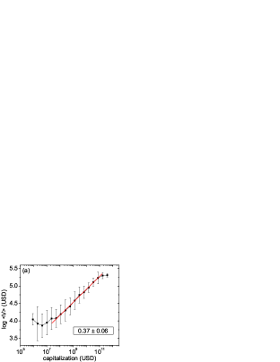
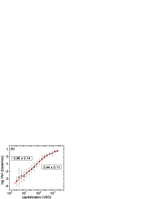
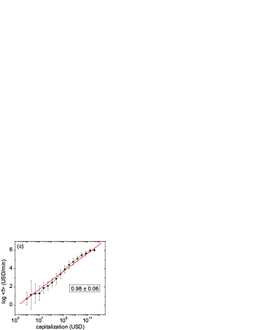
Figure 1: Capitalization dependence of certain measures of trading activity in the year $2000$. The graphs are monotonically increasing and are (piecewise) well approximated by power laws as indicated. All three tendencies curve downward for large capitalizations. (a) Mean value per trade $\left\langle V\right\rangle$ in USD. The fitted slope corresponds to the regime $5\cdot 10^{7}<C<7.5\cdot 10^{10}$ in USD. (b) Mean number of trades per minute $\left\langle N\right\rangle$. The slope on the left is from a fit to $C<4.5\cdot 10^{9}$ USD, while the one on the right is for $C>4.5\cdot 10^{9}$ USD. (c) Mean trading activity (exchanged value per minute) $\left\langle f\right\rangle$ in USD. The plots include $3347$ stocks that were continuously available at NYSE during $2000$.

Many previous studies of trading focus on the stocks of large companies. These certainly have the appealing property that price and returns are well defined even on short time scales due to the high frequency of trading. For infrequently traded stocks, there are extended periods without transactions, and thus prices and returns are undefined. In contrast, other quantities regarding the activity of trading, such as traded value/volume or the number of trades can be defined, even for those stocks where they are zero for most of the time.

In this section we extend the study of Zumbach zumbach which concerned companies of the top two orders of magnitude in capitalization at the London Stock Exchange. Instead, we analyze the $3347$ stocks that were traded continuously at NYSE for the year $2000$. This gives us a range of approximately $10^{6}\dots 6\cdot 10^{11}$ USD in capitalization.

Following Ref. zumbach , we quantify the dependence of trading activity on company capitalization $C_{i}$. Mean value per trade $\left\langle V_{i}\right\rangle$, mean number of trades per minute $\left\langle N_{i}\right\rangle$ and mean activity (traded value per minute) $\left\langle f_{i}\right\rangle$ are plotted versus capitalization in Fig. 1. Ref. zumbach found that all three quantities have power law dependence on $C_{i}$, however, this simple ansatz does not seem to work for our extended range of stocks. While mean trading activity can be approximated as $\left\langle f_{i}\right\rangle\propto C_{i}^{0.98\pm 0.06}$ to an acceptable quality, neither $\left\langle V\right\rangle$ nor $\left\langle N\right\rangle$ can be fitted by a single power law in the whole range of capitalization. Nevertheless, there is – not surprisingly – a monotonic dependence: higher capitalized stocks are traded more intensively.

One can gain further insight from Fig. 2, which shows, that for the largest $1600$ stocks

$$\left\langle V_{i}\right\rangle\propto\left\langle N_{i}\right\rangle^{\beta}$$ (3)

with $\beta=0.57\pm 0.09$. The estimate based on the results of Zumbach zumbach for the stocks in London’s FTSE-100, is $\beta\approx 1$. Similar results were recently obtained for NASDAQ eisler.unified .

For the smaller stocks there is no clear tendency. This effect can be interpreted as follows. As we move to stocks with smaller and smaller capitalization, the average transaction size $\left\langle V\right\rangle$ cannot decrease indefinitely. Transaction costs must impose a minimal number/value of stocks in a single transaction that can still be exchanged profitably. This minimal size is observed as the constant regime for small $\left\langle N\right\rangle$. On the other hand, once a stock is exchanged more frequently (the crossover happens at about $\left\langle N\right\rangle=0.05$ trades/min), it is no more traded in this "minimal" unit. With the growing speed of trading, trades tend to "stick together", it is possible to exchange larger packages. This increase is clear, but not dramatic, it is up to one order of magnitude. Although increasing package sizes reduce transaction costs, price impact gabaix.powerlaw ; plerou.powerlaw ; farmer.powerlaw ; farmer.whatreally increases, possibly decreasing profits and thus limiting package sizes. The interplay of these two effects has a role in the formation of relationship (3).

3 Traded value distributions revisited

The statistical properties of the trading volume of stocks has previously been investigated in Ref. gopi.volume . That work finds that the cumulative distribution of traded volume in $\Delta t=15$ minute windows has a power-law tail with a tail exponent $\lambda=1.7\pm 0.1$. This is the so called inverse half cube law. Formally, this corresponds to

$${\mathbb{P}}_{\Delta t}(f)\propto f^{-(\lambda+1)},$$ (4)

where $\mathbb{P}_{\Delta t}$ is the probability density function of traded volume (value) on a time scale $\Delta t$.

Ever since, great effort was devoted to explain this exponent in terms of the inverse cube law of stock returns gopi.inversecube ; gabaix.powerlaw ; plerou.powerlaw . However, the exact distribution and the possible exponents are still much debated farmer.powerlaw ; queiros.volume , and it has been shown that the shape of such a distribution depends systematically on the capitalization of the company lillo.variety .

The estimation of the tail exponent is a delicate matter. Following the methodology of Ref. gopi.volume – and for the same $1994-1995$ period of data – we repeated these measurements. Our results for the $\Delta t=15$ min distribution are shown in Fig. 3 for three majors stocks. The tails of these distributions can be fitted by a power law over an order of magnitude, for the top $5-10\%$ of the events. The exponent $\lambda$ we find, is significantly higher than $1.7$, it is around $2.2$ for these examples.

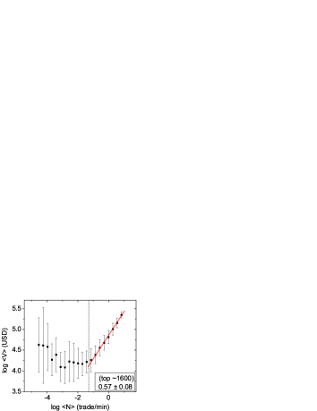
Figure 2: Plot of mean value per trade $\left\langle V\right\rangle$ versus mean number of trades per minute $\left\langle N\right\rangle$ for the year $2000$ of NYSE. For smaller stocks there is no clear tendency. For the top $\sim 1600$ companies ($\left\langle N\right\rangle>0.05$ trades/min), however, there is scaling with an exponent $\beta=0.57\pm 0.08$. Note: The plot includes $3347$ stocks that were continuously available at NYSE during $2000$. Note: The first few points correspond to stocks that are traded less than daily. These typically do not represent individual companies and might be traded according to different rules. However, unlike prices or returns, $V$, $N$ and $f$ still remain well-defined quantities for such stocks.

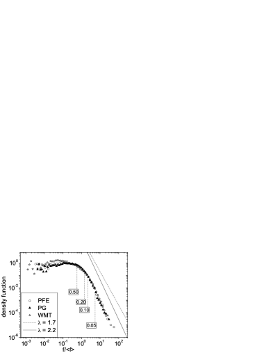
Figure 3: Distributions of traded value in $\Delta t=15$ min time windows, divided by the mean. The plot displays three example stocks for the period $1994-1995$. The numbers show some upper quantiles of the distribution (probability of values higher than indicated by the corresponding dashed line). The dashed and solid diagonal lines represent power-laws with exponents corresponding to $\lambda=1.7$ and $2.2$, respectively.

For systematic calculations of $\lambda$, there is a range of mathematical tools available. We used three variants of Hill’s method hill ; alves to estimate the tail exponent, details can be found in Appendices A and B. All three have a common parameter: the number $k$ of largest events that belong to the tail. The statistical weight associated with the tail events is $p=k/L$, where $L$ is the total length of our time series. From Fig. 3 one can see, that $p\approx 5-10\%$ is the proper choice as a threshold for the asymptotic regime.

For the two-year period $1994-1995$ and separately for the single year $2000$, we took the $1000$ stocks with the highest total traded value in the TAQ database. We detrended their trading activity by the well known $U$-shaped intraday pattern (see, e.g., Ref. eisler.non-universality ). Then, we calculated the distribution of $\lambda$ over these stocks. The median and the width of this distribution (characterized by the half distance of the $25\%$ and $75\%$ quantiles) is shown in Tables 1 and 2 for various time windows $\Delta t$.

The choice $p=0.06$ in Hill’s method provides results in line with Ref. gopi.volume . For $\Delta t=15$ min time windows, one finds $\lambda=1.71\pm 0.20$ for the period $1994-1995$. However, other estimates are significantly higher, $\lambda>2$. Moreover, two estimators show a strong tendency of increasing $\lambda$ with increasing time windows. Monte Carlo simulations on surrogate datasets show, that this is beyond what could be explained by decreasing sample size. It is well known, that for $\lambda<2$ the distribution would have to converge to the corresponding Levy distribution when $\Delta t\rightarrow\infty$. The measured $\lambda$’s should also be independent of $\Delta t$. On the other hand, for $\lambda>2$, the $\Delta t\rightarrow\infty$ limit distribution is a Gaussian. Accordingly, for finite samples, the measured effective value of $\lambda$ increases with $\Delta t$. This systematic dependence makes us conclude that there is a strong indication for the existence of the second moment.

One must keep in mind, that all three methods assume that the variable is asymptotically distributed as (4) and none of them proves it. If this does not hold, then the estimates of exponents are only a parametric characterization of the unknown functional form, nevertheless, they do suggest that the second moments exist. If the distribution is indeed of the limiting form (4), then although for short time windows ($\Delta t<60$ min) there is a fraction of stocks whose estimate gives $\lambda<2$, even those display $\lambda>2$ for larger $\Delta t$.

Based on these results we conclude that the second moments of the distribution must exist for any $\Delta t$, therefore the calculation of the Hurst exponent for the related time series is meaningful. Similar qualitative features were found for the years $2001$ and $2002$ uponrequest .

$\Delta t$	Hill’s method ($p=0.06$)	Shifted Hill’s $\lambda$	Shifted Hill’s $\varphi$	Fraga Alves ($p=0.1$)
$1$ min	$1.43\pm 0.09$	$2.15\pm 0.15$	$3.0$	$1.98\pm 0.25$
$5$ min	$1.56\pm 0.13$	$2.29\pm 0.25$	$2.8$	$2.04\pm 0.25$
$15$ min	$1.71\pm 0.20$	$2.55\pm 0.35$	$2.8$	$2.1\pm 0.3$
$60$ min	$2.06\pm 0.30$	$2.85\pm 0.45$	$1.8$	$2.1\pm 0.4$
$120$ min	$2.3\pm 0.4$	$3.15\pm 0.70$	$1.6$	$2.1\pm 0.4$
$390$ min	$2.7\pm 0.6$	$3.7\pm 0.9$	$1.2$	no estimate

Table 1: Median of the tail exponents of traded value calculated by three methods for $1994-1995$. The width of the distributions is given with the half distance of the $25\%$ and $75\%$ quantiles.

$\Delta t$	Hill’s method ($p=0.06$)	Shifted Hill’s $\lambda$	Shifted Hill’s $\varphi$	Fraga Alves ($p=0.1$)
$1$ min	$1.63\pm 0.13$	$2.40\pm 0.23$	$2.6$	$2.16\pm 0.25$
$5$ min	$1.91\pm 0.25$	$2.8\pm 0.5$	$2.4$	$2.30\pm 0.35$
$15$ min	$2.15\pm 0.40$	$3.1\pm 0.6$	$2.0$	$2.35\pm 0.40$
$60$ min	$2.6\pm 0.5$	$3.45\pm 0.8$	$1.2$	$2.2\pm 0.4$
$120$ min	$2.8\pm 0.6$	$3.8\pm 1.1$	$1.2$	no estimate
$390$ min	$3.2\pm 1.0$	$5.1\pm 0.8$	$1.6$	no estimate

Table 2: Median of the tail exponents traded value calculated by three methods for $2000$. The width of the distributions is given with the half distance of the $25\%$ and $75\%$ quantiles.

4 Non-universality of correlations in traded value time series

Scaling methods vicsek.book ; dfa.intro ; dfa have long been used to characterize a wide variety of time series, including stock prices and trading volumes bouchaud.book ; stanley.book . In particular, the Hurst exponent $H(i)$ is usually calculated. For the traded value time series $f_{i}^{\Delta t}(t)$ of stock $i$, it is defined as

$$\sigma_{i}^{2}(\Delta t)=\left\langle\left(f_{i}^{\Delta t}(t)-\left\langle f_{i}^{\Delta t}(t)\right\rangle\right)^{2}\right\rangle\propto\Delta t^{2H(i)},$$ (5)

where the average is taken over the time variable $t$. As discussed in Sec. 3, the variance on the left hand side exists for any stock or time scale $\Delta t$.

Ref. gopi.volume finds strong correlations in $\sqrt{f_{i}^{\Delta t}(t)}$ with $H\approx 0.83$. Their analysis comprises the $1000$ largest companies in the period $1994-1995$ and they use $\Delta t>1$ day except for some very frequently traded stocks.

We extend these measurements to all $2647$ stocks that were continuously traded in the period $2000-2002$. The time series display a crossover from a lower to a higher value of $H(i)$ around the time scale of one day (for an example, see the inset of Fig. 4). A similar effect was reported for intertrade times of large companies ivanov.itt . Intraday correlations are not meaningful for some of the smallest companies as their shares are often not exchanged for several days. Nevertheless, for any choice of time windows, one recovers a tendency: With the change of average traded value $\left\langle f_{i}\right\rangle$, there is a clear logarithmic trend in the Hurst exponent, especially above the daily scale:

$$H(i)=H(i=1)+\gamma\log\left\langle f_{i}\right\rangle,$$ (6)

where normalization is so that $\left\langle f_{i=1}\right\rangle=1$. Measurement results and values of $\gamma$ are given in Fig. 4. Calculations for the periods $1994-1995$ and $1998-1999$ show qualitatively similar properties. On the grounds of a new type of scaling law eisler.non-universality , this effect can be predicted analytically eisler.unified . Here we only focus on the description of the phenomenon.

Trading activity of very small stocks shows nearly no persistence. Even for $\Delta t>1$ day, $H\approx 0.5$. This changes as one moves to larger and larger companies. Their trading can be more correlated in the regime $\Delta t>1$ day, up to $H\approx 0.9$. This is a clear sign of non-universality. The very nature of trading differs for different company sizes and statistics such as "distributions of Hurst exponents" is meaningless. No typical value exists, the trend is systematic and continuous. As Hurst exponents are closely related to the multifractal spectra vicsek.book ; ball.falpha of $f$, those cannot be universal either. This raises doubts about an "average multifractal spectrum" as calculated in, e.g., Ref. drozdz.average .

Systematic dependence of the exponent of the power spectrum of the number of trades on capitalization was previously reported in Ref. bonanno.dynsec , based on the study of $88$ stocks. This quantity is closely related to the Hurst exponent for the time series of the number of trades per unit time (see Ref. ivanov.itt ). Direct analysis finds a strong dependence of the Hurst exponent of $N$ on $\left\langle N\right\rangle$, but no such clear logarithmic trend as Eq. (6) uponrequest .

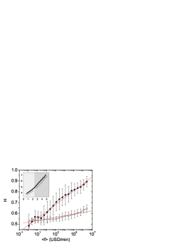
Figure 4: The Hurst exponent of traded value $f$ shows logarithmic dependence on the average traded value per minute $\left\langle f\right\rangle$. For intraday fluctuations ($\Circle$), correlations in $\left\langle f\right\rangle$ are weak, $H\approx 0.5-0.6$, the fitted slope is $\gamma(\Delta t<\mathrm{250min})=0.016\pm 0.001$. Beyond the daily scale ($\blacksquare$) the effect increases: the smallest stocks show almost no correlation ($H\approx 0.5$), while large ones display strong persistence ($H\approx 0.9$). The fitted slope is $\gamma(\Delta t>\mathrm{630min})=0.063\pm 0.002$. The inset shows the two regimes of correlation strength for the single stock Wal-Mart (WMT) on a log-log plot of $\sigma(\Delta t)$ versus $\Delta t$. The slopes corresponding to Hurst exponents are $0.65$ and $0.8$.

5 Multiscaling distribution of intertrade times

Finally, we analyzed the intertrade interval series $T_{i}(n=1\dots N_{i}-1)$, defined as the time spacings between the $n$’th and $n+1$’th trade scalas.anomalous . $N_{i}$ is the total number of trades for stock $i$ during the period under study.

Previously, Ref. ivanov.itt used $30$ stocks from the TAQ database for the period $1993-1996$ and proposed that the distribution of $T_{i}$ scales with the mean $\left\langle T_{i}\right\rangle$ as

$$\mathbb{P}(T,\left\langle T\right\rangle)=\frac{1}{\left\langle T\right\rangle}F(T/\left\langle T\right\rangle),$$ (7)

and the universal scaling function $F$ is well modeled by a Weibull distribution of the form

$$F(x)=\frac{\delta}{X}\left(\frac{x}{X}\right)^{\delta-1}\exp\left[-\left(\frac{x}{X}\right)^{\delta}\right],$$ (8)

where $X\approx 0.94$ and $\delta\approx 0.72$ for all the $30$ stocks, with some statistical deviations.

We analyzed the data by including a large number of stocks with very different capitalizations. First it has to be noted that the mean intertrade interval has decreased drastically over the years. In this sense the stock market cannot be considered stationary for periods much longer than one year. We analyze the two year period $1994-1995$ (part of that used in Ref. ivanov.itt ) and separately the single year $2000$. We use all stocks in the TAQ database with $\left\langle T\right\rangle<10^{5}$ sec, a total of $3924$ and $4044$ stocks, respectively.

In order to check the validity of the gap scaling formula, we divided the stocks into two groups with respect to $\left\langle T\right\rangle$. Then, we generated the distribution of $T/\left\langle T\right\rangle$ for the groups, a comparison for the year $2000$ is shown in Figure 5. This already raises doubts about the generality of Eq. (8): The tails of the distribution seem to possess more weight for the group with small $\left\langle T\right\rangle$ (blue chips). The direct visual comparison of these distributions is, however, not always a reliable method to evaluate universality. Instead, we take a less arbitrary, indirect approach.

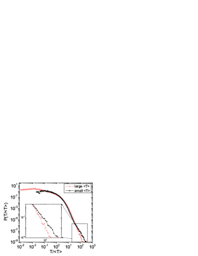
Figure 5: The distribution of $T/\left\langle T\right\rangle$ in the year $2000$ for two groups of stocks with different mean intertrade times $\left\langle T\right\rangle$. The group with the most frequently traded stocks (blue chips) has a considerably greater weight for waiting times. This implies that the distribution $\mathbb{P}(T,\left\langle T\right\rangle)$ may not be universal.

The consequence of the universal distribution (7) would be that the moments of $T$ should show gap scaling: The difference between the exponents of the $q$-th and $q+1$-th moments is independent of $q$. halsey.strange ; murthy.sinai :

$$\left\langle T_{i}^{q}\right\rangle=C(q)\left\langle T_{i}\right\rangle^{-\tau(q)},$$ (9)

with a scaling function $-\tau(q)\equiv q$.

Instead, we find a systematic dependence of $-\tau$ on $q$, see Fig. 6 for several examples of fitting and Fig. 7 for all results. There is good fit to a power law of type (9) for $4$ orders of magnitude in $\left\langle T\right\rangle$ with non-trivial exponents.

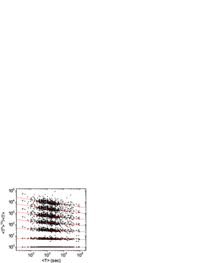
Figure 6: Scaling of integer moments of $T$, $q=1,2,4,6,8,12,16$ (increasing from bottom to top). The plot shows $\left\langle T^{q}\right\rangle^{1/q}/\left\langle T\right\rangle$, the slopes correspond to $-\tau(q)/q-1$. If the normalized distribution of $T$ were universal, the points would align on horizontal lines. Note: The points were shifted vertically for better visibility. Only $400$ points are shown per moment, the sample period was $1994-1995$.

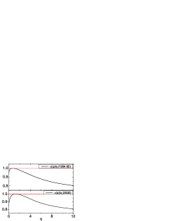
Figure 7: Scaling exponents for the moments of intertrade interval distributions defined in Eq. (9). The values $-\tau(q)\equiv q$ would imply a universal distribution that is independent of stock. The fact that $-\tau(q)/q<1$, shows less frequently traded stocks display relatively lower variations in their trading dynamics. For large $q$, the effect increases monotonically with $q$. This suggests a difference between small and large stocks in the tail of the distribution, which corresponds to longer periods of inactivity.

The intuitive meaning of $-\tau(q\gg 1)<q$ is simple: Intertrade times of larger (more frequently traded) stocks exhibit larger relative fluctuations. In line with our observation from Figure 5, this difference must come from the tail of the distribution, as the deviation becomes more pronounced for higher moments.

The absence of simple universal scaling raises the question of the capitalization dependence of the Hurst exponent for the time series $T_{i}$, defined analogously to Eq. (5) as

$$\sigma_{i}^{2}(N)=\left\langle\left(\sum_{n=1}^{N}T_{i}(n)-\left\langle\sum_{n=1}^{N}T_{i}(n)\right\rangle\right)^{2}\right\rangle\propto N^{2H_{T}(i)}.$$ (10)

The data show a crossover, similar to that for the traded value $f$, from a lower to a higher value of $H_{T}(i)$ when the window size is approximately the daily mean number of trades (for an example, see the inset of Fig. 8). For the restricted set studied in Ref. ivanov.itt , the value $H_{T}\approx 0.94\pm 0.05$ was suggested for window sizes above the crossover.

Much similarly to the case of traded value Hurst exponents analyzed in Section 4, the inclusion of more stocks reveals the underlying systematic non-universality. Again, less frequently traded stocks appear to have weaker autocorrelations as $H_{T}$ decreases monotonically with growing $\left\langle T\right\rangle$. One can fit an approximate logarithmic law ^, to characterize the trend:

$$H_{T}=H_{T}(\left\langle T\right\rangle=1)+\gamma_{T}\log\left\langle T\right\rangle,$$ (11)

where $\gamma_{T}=-0.10\pm 0.02$ for the period $1994-1995$ (see Fig. 8) and $\gamma_{T}=-0.08\pm 0.02$ for the year $2000$ uponrequest .

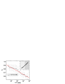
Figure 8: Hurst exponents of $T_{i}$ for time windows greater than $1$ day, plotted versus the mean intertrade time $\left\langle T_{i}\right\rangle$. Stocks that are traded less frequently, show markedly weaker persistence of $T$ for time scales longer than $1$ day. The dotted horizontal line serves as a reference. We used stocks with $\left\langle T\right\rangle<10^{5}$ sec, the sample period was $1994-1995$. The inset shows the two regimes of correlation strength for the single stock General Electric (GE) on a log-log plot of $\sigma(N)$ versus $N$. The slopes corresponding to Hurst exponents are $0.6$ and $0.89$.

In their recent preprint, Yuen and Ivanov ivanov.unpublished independently show a tendency similar to Eq. (11) for intertrade times of NYSE and NASDAQ in a different set of stocks.

6 Conclusions

In this paper we revisited some “stylized facts” of stock market data and found in several ways alterations from earlier conclusions. The main difference in our approach was – besides the comparative application of extrapolation techniques – the extension of the range of capitalization of the studied firms. This enabled us to investigate the dependence of the trading characteristics on capitalization itself. In fact, in many cases we found fundamental dependence on this parameter.

We have shown that trading activity $\left\langle f\right\rangle$, the number of trades per minute $\left\langle N\right\rangle$ and the mean size of transactions $\left\langle V\right\rangle$ display non-trivial, but monotonic dependence on company capitalization.

We have given evidence that the distribution of traded value in fixed time windows is not Levy stable. If a power law is fitted to the tail of the distribution, a careful analysis yields to an exponent $\lambda$, which is – even for short time windows – in most cases greater than $2$, and then increases with increasing time window indicating the existence of the second moment of the distribution. Consequently, the Hurst exponent $H$ for its variance can be defined and it depends on the mean trading activity $\left\langle f\right\rangle$ as

$$H(i)=H(i=1)+\gamma\log\left\langle f_{i}\right\rangle.$$

The mean transaction size can be fitted to a power-law dependence on the trading frequency for moderate to large companies.

The distribution of the waiting times between trades is better described multiscaling than by gap scaling. It is characterized by an increase in both correlations and relative fluctuations with growing trading frequency (i.e. increasing capitalization).

Our findings indicate that special care must be taken when concepts like scaling and universality are applied to financial processes. The modeling of the market should be extended to the capitalization dependence of the characteristic quantities and this seems a real challenge at present.

Appendix A The estimation of tail exponents $\lambda$

In the following, for every measurement we give the median estimates of $\lambda$ for the $1000$ stocks with highest traded value during the investigated period. The error bars show the half distance between the $25\%$ and $75\%$ quantiles of $\lambda$.

A.1 Hill’s estimator

Hill’s estimator [22] is a statistically consistent method to estimate the tail exponent $\lambda$ from random samples taken from a distribution that asymptotically has the power-law form (4). The procedure first sorts the sample $f(t=1\dots L)$ in decreasing order. We are going to denote this series by $f[t]$, so that $f[1]>f[2]>f[3]>\dots$. Then, one defines the tail of the distribution by setting an arbitrary number $k$ of points to be included in the estimation procedure. The estimate of the inverse tail exponent is

$$\hat{\lambda}^{-1}(k)=\left[\frac{1}{(k-1)}\sum_{t=1}^{k-1}\log f[t]\right]-\log f[k],$$ (12)

given that $k\rightarrow\infty$ and $p=k/L\rightarrow 0$. If the sampled distribution is of the form (4), then by increasing $k$, the estimator converges rapidly to the actual value of $\lambda^{-1}$. However, in the case of traded value data, this turns out not to be the case.

The inset of Fig. 9(a) – a so called Hill plot – shows, that there is a systematic dependence of $\lambda$ on $p$ and no convergence is observed. With the inclusion of less tail events, the exponent increases sharply, beyond the $\lambda=2$ threshold for Lévy stability. Further evidence for the lack of Lévy stability is that on increasing the time scale $\Delta t$, the estimated tail exponents also increase further as shown in Fig. 9(a).

This type of behavior is not new to mathematical statistics (see, e.g., Ref. [23]). It is possible, that the distribution decays faster than a power law and thus no finite $\lambda$ exists. Alternatively, the power law may not be centered around zero, but instead it can be of the form

$${\mathbb{P}}_{\Delta t}(f)\propto\left(f+f_{0}\right)^{-(\lambda+1)}.$$ (13)

In this latter case, there is a finite $\lambda$, but as the sample size $T$ is usually too small, the estimator displays the above bias. One can either try to approximate the value of $f_{0}$ and shift the data accordingly, so that Hill’s estimator converges properly, or try to find another estimator that is insensitive to this shifting constant.

We have tried both approaches and they yielded qualitatively similar results.

A.2 Shifted Hill’s estimator

One can apply Hill’s estimator to the points $f[t=1\dots L]+\varphi\left\langle f\right\rangle$, where $\varphi$ is a constant parameter and look for a value, where the estimator $\lambda(k)$ becomes independent of $k$, i.e., Hill’s estimator truly finds a power-law decay that is now consistent with Eq. (13). For an example, see Fig. 9(a). This happens, when $\varphi\left\langle f\right\rangle=f_{0}$. How this shift by $\varphi\left\langle f\right\rangle$ affects the Hill plots is shown in Fig. 9(c) for the case of $\Delta t=15$ min. One finds, that in this case $\varphi\approx 2.8$ gives reasonable results, while $\lambda=2.55\pm 0.35$. One can repeat the procedure for various time scales $\Delta t$. The median Hill plots are shown in Fig. 9(d), while $\lambda(\Delta t)$ and $\varphi(\Delta t)$ are given in Table 1. Again, one finds a significant increase of the tail exponent with growing $\Delta t$. This underlines our previous expectation that traded value distributions are not Lévy stable and thus have a finite variance.

   

        

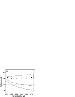
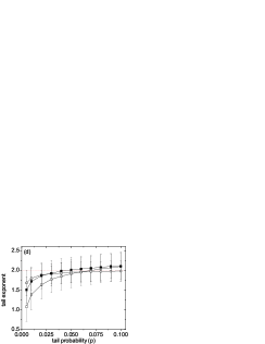
Figure 9: (a) Hill’ s estimates of $\lambda$ for different sizes of the time window with the tail probability set as $p=0.06$. The monotonic trend indicates that the distribution is not be Levy stable. The inset shows, that for $\Delta t=15$ min the effective tail exponent $\lambda$ depends monotonically on the choice for tail probability $p$. Thus, Hill’s estimates are unreliable, because they depend strongly on an arbitrary parameter. (b) Dependence of the Hill plots for $\Delta t=15$ min on the shifting constant $\varphi$. The values of $\varphi$ from bottom to top: $0$ ($\Box$), $1$ ($\bigtriangleup$), $2.8$ ($\CIRCLE$, optimal shift), $3.0$ ($\Circle$). Typical error bars are given on the right, darker gray indicates the regimes where they overlap. (c) Hill plots of the optimally shifted Hill’s estimators for various time windows. The values of $\Delta t$ from bottom to top: $1$ min ($\blacksquare$), $5$ min ($\CIRCLE$), $15$ min ($\blacktriangle$), $60$ min ($\blacktriangledown$), $120$ min ($\blacklozenge$), $390$ min ($\bigstar$). One finds $\lambda>2$ and the strong increasing tendency in $\lambda$ with $\Delta t$ implies that the distribution is not Levy stable. (d) Hill plots of the Fraga Alves estimator for three time window sizes $\Delta t$: $1$ min ($\Circle$), $15$ min ($\blacksquare$), $60$ min ($\Box$). The method gives a lower estimate of $\lambda\approx 2$.

A.3 Fraga Alves estimator

A more sophisticated approach to estimate tail exponents of distributions of the type (13), is a recent variant of Hill’s method, proposed by Fraga Alves [23]. The algorithm is described in detail in Appendix B and its estimates of $\lambda$ are – in an exact mathematical sense – independent of the shift $f_{0}$ present in the density function, unlike those of the original Hill’s estimator (12).

We applied the estimator to the same dataset, the Hill plots for $\Delta t=1,15,60$ min are shown in Fig. 9(d). What one finds is a very different behavior from the shifted Hill’s estimator. The estimate of $\lambda$ increases with growing $p$, i.e., the more points included. This is due to that the Fraga Alves estimator converges much slower than Hill’s estimator, and – as Fig. 9(d) and Monte Carlo simulations on surrogate datasets indicate – it converges from below. On the other hand, setting the threshold as high as $p=0.1$ may include events that no more belong to the power law regime, which also results in a reduced, effective exponent due to the shape of the distribution, shown in Fig. 3. Consequently, this method provides a lower estimate of $\lambda$. Still, the calculated values are mostly above $2$. Finally, one must note that for $\Delta t\geq 120$ min, the number of points was inadequate to provide any proper estimate at all.

Appendix B The algorithm of the Fraga Alves estimator

Ref. [23] describes a method to approximate the parameter $\lambda$ from a sample of a random variable that is asymptotically distributed as

$$\mathbb{P}_{\Delta t}(f)\propto(f+f_{0})^{-(\lambda+1)}.$$

First, one sorts the sample $f(t=1\dots L)$ in decreasing order. We denote this series by $f[t]$, so that $f[1]>f[2]>f[3]>\dots$. Then, the procedure consists of the five steps formulated below:

1. $k_{0}^{*}=2k^{2/3}$

2. $$\hat{\lambda}^{-1}(k_{0}^{*},k)=\frac{1}{k_{0}^{*}-1}\sum_{t=1}^{k_{0}^{*}-1}\log\frac{f[t]-f[k]}{f[k_{0}]-f[k]}$$

3. $$k_{0}=C_{0}^{1/(2\hat{\lambda}^{-1}(k_{0}^{*},k)+1)}k^{\alpha},$$

   where

   $$C_{0}=\frac{(1+\hat{\lambda}^{-1}(k_{0}^{*},k))^{2}}{2\hat{\lambda}^{-1}(k_{0}^{*},k)},$$

   and

   $$\alpha=\frac{2\hat{\lambda}^{-1}(k_{0}^{*},k)}{2\hat{\lambda}^{-1}(k_{0}^{*},k)+1}.$$

4. $$\hat{\lambda}^{-1}(k_{0},k)=\frac{1}{k_{0}-1}\sum_{t=1}^{k_{0}-1}\log\frac{f[t]-f[k]}{f[k_{0}]-f[k]}$$

5. Finally, the estimate of the inverse tail exponent is given by

   $$\lambda^{-1}(k_{0},k)=\hat{\lambda}^{-1}(k_{0},k)-\sqrt{\frac{\hat{\lambda}^{-1}(k_{0},k)}{2k_{0}}}.$$

   $\lambda^{-1}(k_{0},k)$ converges to the inverse tail exponent, if $L\rightarrow\infty$, $k/L\rightarrow 0$ and $k_{0}/k\rightarrow 0$.

References

- [1] P.W. Anderson, editor. The Economy As an Evolving Complex System (Santa Fe Institute Studies in the Sciences of Complexity Proceedings), 1988.
- [2] W.B. Arthur, S.N. Durlauf, and D.A. Lane, editors. The Economy As an Evolving Complex System II: Proceedings (Santa Fe Institute Studies in the Sciences of Complexity Lecture Notes), 1997.
- [3] J. Kertész and I. Kondor, editors. Econophysics: An Emergent Science, http://newton.phy.bme.hu/kullmann/Egyetem/ konyv.html. 1997.
- [4] J.-P. Bouchaud and M. Potters. Theory of Financial Risk. Cambridge University Press, Cambridge, 2000.
- [5] R.N. Mantegna and H.E. Stanley. Introduction to Econophysics: Correlations and Complexity in Finance. Cambridge University Press, 1999.
- [6] B.B. Mandelbrot. Fractals and scaling in finance: Discontinuity, concentration, risk. 1997.
- [7] L.E. Reichl. A Modern Course in Statistical Physics, 2nd edition. Wiley, 1998.
- [8] P. Gopikrishnan, M. Meyer, L.A.N. Amaral, and H.E. Stanley. Inverse cubic law for the distribution of stock price variations. Eur. Phys. J. B, 3:139–140, 1998.
- [9] T. Lux. The stable paretian hypothesis and the frequency of large returns: An examination of major german stocks. Applied Financial Economics, 6:463–475, 1996.
- [10] M. Gallegatti, S. Keen, T. Lux, and P. Ormerod. Worrying trends in econophysics. http://www.unifr.ch/econophysics, doc/0601001; to appear in Physica A, Proceedings of the World Econophysics Colloquium, Canberra, 2005.
- [11] P. Gopikrishnan, V. Plerou, X. Gabaix, and H.E. Stanley. Statistical properties of share volume traded in financial markets. Phys. Rev. E, 62:4493–4496, 2000.
- [12] P.Ch. Ivanov, A. Yuen, B. Podobnik, and Y. Lee. Common scaling patterns in intertrade times of U.S. stocks. Phys. Rev. E, 69:56107, 2004.
- [13] Trades and Quotes Database for 1993-2003, New York Stock Exchange, New York.
- [14] G. Zumbach. How trading activity scales with company size in the FTSE 100. Quantitative Finance, 4:441–456, 2004.
- [15] Z. Eisler and J. Kertész. Scaling theory of temporal correlations and size dependent fluctuations in the traded value of stocks. Phys. Rev. E, 73:046109, 2006.
- [16] X. Gabaix, P. Gopikrishnan, V. Plerou, and H.E. Stanley. A theory of power-law distributions in financial market fluctuations. Nature, 423:267–270, 2003.
- [17] V. Plerou, P. Gopikrishnan, X. Gabaix, and H.E. Stanley. On the origin of power-law fluctuations in stock prices. Quantitative Finance, 4:C11–C15, 2004.
- [18] J.D. Farmer and F. Lillo. On the origin of power law tails in price fluctuations. Quantitative Finance, 4:C7–C11, 2004.
- [19] J.D. Farmer, L. Gillemot, F. Lillo, S. Mike, and A. Sen. What really causes large price changes? Quantitative Finance, 4:383–397, 2004.
- [20] S.M.D. Queirós. On the distribution of high-frequency stock market traded volume: a dynamical scenario. Europhys. Lett., 71:339–345, 2005.
- [21] F. Lillo and R.N. Mantegna. Variety and volatility in financial markets. Phys. Rev. E, 62:6126–6134, 2000.
- [22] B.M. Hill. A simple general approach to inference about the tail of a distribution. Annals of Statistics, 3:1163–1174, 1975.
- [23] M.I. Fraga Alves. A location invariant hill-type estimator. Extremes, 4:199–217, 2001.
- [24] Z. Eisler, J. Kertész, S.-H. Yook, and A.-L. Barabási. Multiscaling and non-universality in fluctuations of driven complex systems. Europhys. Lett., 69:664–670, 2005.
- [25] Data available upon request.
- [26] T. Vicsek. Fractal Growth Phenomena. World Scientific Publishing, 1992.
- [27] C.-K. Peng, S.V. Buldyrev, S. Havlin, M. Simons, H.E. Stanley, and A.L. Goldberger. Mosaic organization of DNA nucleotides. Phys. Rev. E, 49:1685–1689, 1994.
- [28] J.W. Kantelhardt, S.A. Zschiegner, E. Koscielny-Bunde, S. Havlin, A. Bunde, and H. Eugene Stanley. Multifractal detrended fluctuation analysis of nonstationary time series. Physica A, 316:87–114, 2002.
- [29] R.C. Ball and O.R. Spivack. The interpretation and measurement of the spectrum of a multifractal measure. J. Phys. A: Math. Gen., 23:5295–5307, 1990.
- [30] J. Kwapien, P. Oswiecimka, and S. Drozdz. Physica A, 350:466–474, 2005.
- [31] G. Bonanno, F. Lillo, and R.N. Mantegna. Dynamics of the number of trades of financial securities. Physica A, 280:136–141, 2000.
- [32] E. Scalas, R. Gorenflo, H. Luckock, F. Mainardi, M. Mantelli, and M. Raberto. Anomalous waiting times in high-frequency financial data. Quantitative Finance, 4:695–702, 2004.
- [33] T.C. Halsey, M.H. Jensen, L.P. Kadanoff, I. Procaccia, and B.I. Shraiman. Fractal measures and the singularities: The characterization of strange sets. Phys. Rev. A, 33:1141–1151, 1986.
- [34] K.P.N. Murthy, K.W. Kehr, and A. Giacometti. Multifractal scaling of moments of mean first-passage time in the presence of Sinai disorder. Phys. Rev. E, 53:444–449, 1996.
- [35] A. Yuen and P.Ch. Ivanov. Impact of stock market microstructure on intertrade time and price dynamics. arXiv:physics/0508203, 2005.
Acknowledgements.
The authors are indebted to Vasiliki Plerou and Parameswaran Gopikrishnan for discussions on Hill’s method and Géza Györgyi for his insights on correlated time series. They also thank György Andor and Ádám Zawadowski for their support with the data. Finally, they would like to thank Plamen Ch. Ivanov for calling their attention to some recent results on market dynamics. JK is member of the Center for Applied Mathematics and Computational Physics, BME; furthermore, he is grateful for the hospitality of Dietrich Wolf (Duisburg) and of the Humboldt Foundation. Support by OTKA T049238 is acknowledged.Appendix A The estimation of tail exponents