Simple estimation of absolute free energies for biomolecules

Abstract

One reason that free energy difference calculations are notoriously difficult in molecular systems is due to insufficient conformational overlap, or similarity, between the two states or systems of interest. The degree of overlap is irrelevant, however, if the absolute free energy of each state can be computed. We present a method for calculating the absolute free energy that employs a simple construction of an exactly computable reference system which possesses high overlap with the state of interest. The approach requires only a physical ensemble of conformations generated via simulation, and an auxiliary calculation of approximately equal central-processing-unit (CPU) cost. Moreover, the calculations can converge to the correct free energy value even when the physical ensemble is incomplete or improperly distributed. As a “proof of principle,” we use the approach to correctly predict free energies for test systems where the absolute values can be calculated exactly, and also to predict the conformational equilibrium for leucine dipeptide in implicit solvent.

I Introduction

Knowledge of the free energy for two different states or systems of interest allows the calculation of solubilities, grossfield-jacs; vangunsteren-onestep determines binding affinities of ligands to proteins, kollman-pnas; vangunsteren-estrogen and determines conformational equilibria (e.g., Ref. ytreberg-shift). Free energy differences ($\Delta F$) therefore have potential application in structure-based drug design where current methods rely on ad hoc protocols to estimate binding affinities. shoichet-nature; scheraga

Poor “overlap,” the lack of configurational similarity between the two states or systems of interest, is a key cause of computational expense and error in $\Delta F$ calculations. The most common approach to improve overlap in free energy calculations (used in thermodynamic integration, and free energy perturbation) is to simulate the system at multiple hybrid, or intermediate stages (e.g., Refs. zwanzig; beveridge; jorgensen; karplus-jcp; mccammon). However, the simulation of intermediate stages greatly increases the computational cost of the $\Delta F$ calculation.

Here, we address the overlap problem by calculating the absolute free energy for each of the end states, thus avoiding the need for any configurational overlap. Our method relies on the calculation of the free energy difference between a reference system (where the exact free energy can be calculated, either analytically or numerically) and the system of interest.

Such use of a reference system with a computable free energy has been used successfully in solids where the reference system is generally a harmonic or Einstein solid, hoover71; frenkel and liquid systems, where the reference system is usually an ideal gas. hoover67; reinhardt-absf The scheme has also been applied to molecular systems by Stoessel and Nowak, using a harmonic solid in Cartesian coordinates as a reference system. stoessel

Other approaches to calculate the absolute free energies of molecules have been developed. Meirovitch and collaborators calculated absolute free energies for peptides in vacuum, for liquid argon and water using the hypothetical scanning method. meirovitch-deca; meirovitch-argon Computational cost has thus far limited the approach to peptides with sixty degrees of freedom. meirovitch-jcp The “mining minima” approach, developed by Gilson and collaborators, estimates the absolute free energy of complex molecules by attempting to enumerate the low-energy conformations and estimating the contribution to the configurational integral for each. gilson-jpca; gilson-bj Anharmonic effects can be included. gilson-jacs The mining minima method can, in principle, include potential correlations between the torsions and bond angles or lengths, and uses an approximate method to compute local partition functions. Other investigators have estimated absolute free energies for molecules using harmonic or quasi-harmonic approximations, karplus-deca; gilson-jacs; aqvist-absf however, as discussed in Refs. gilson-jacs and karplus-deca local minima can be deviate substantially from a parabolic shape.

We introduce, apparently for the first time, a reference system which is constructed to have high overlap with fairly general molecular systems. The approach can make use of either internal or Cartesian coordinates. For biomolecules, using internal coordinates greatly enhances the accuracy of the method since internal coordinates are tailored to the description of conformations. Further, all degrees of freedom and their correlations are explicitly included in the method.

Our method differs in several ways from the important study of Stoessel and Nowak: stoessel (i) we use internal coordinates for molecules which are key for optimizing the overlap between the reference system and the system of interest; (ii) we may use a nearly arbitrary reference potential because only a numerical reference free energy value is needed, not an analytic value; (iii) there is no need, in cases we have studied, to use multi-stage methodology to find the desired free energy due to the overlap built into the reference system,

We consider this report a “proof of principle” for our reference system method. After introducing the method, it is tested on single and double-well two-dimensional systems, and on a methane molecule where absolute free energy estimates can be compared to exact values. The method is then used to compute the absolute free energy of the alpha and beta conformations for leucine dipeptide (ACE-(leu)₂-NME) in implicit solvent, using all one-hundred fifteen degrees of freedom, correctly calculating the free energy difference $\Delta F_{\rm alpha\rightarrow beta}$. Extensions of the method to larger systems are then discussed.

II Reference system method

II.1 The fundamental relations

The absolute free energy of the system of interest (“phys” for physical) is defined using the partition function $Z_{\rm phys}$

$$F_{\rm phys}=-k_{B}T\ln Z_{\rm phys}=$$

$$-k_{B}T\ln\left[\int d\vec{x}\;e^{-\beta\big{(}U_{\rm phys}(\vec{x})+K_{\rm phys}(\vec{x})\big{)}}\right],$$ (1)

where $T$ is the system temperature, $\beta=1/k_{B}T$, $U_{\rm phys}$ and $K_{\rm phys}$ are, respectively, the physical potential energy (i.e., simulation forcefield) and the kinetic energy, and $\vec{x}$ represents the full set of configurational coordinates (internal or Cartesian). The kinetic energy term can be integrated exactly to obtain gilson-jpcb

$$Z_{\rm phys}=\Bigg{[}\frac{1}{h^{3N}}\frac{8\pi^{2}}{\sigma C^{\circ}}\prod_{i=1}^{N}\big{(}2\pi k_{B}Tm_{i}\big{)}^{3/2}\Bigg{]}\int d\vec{x}\;e^{-\beta U_{\rm phys}(\vec{x})},$$ (2)

where $m_{i}$ is the mass of atom $i$, $h$ is Planck’s constant, $C^{\circ}$ is the standard concentration, $\sigma$ is the symmetry number, gilson-bj $N$ is the number of particles in the system, and the integral is defined to be the configurational partition function. For method used in this study the absolute free energy of the system of interest is calculated using a reference system (“ref”), and the following relationships are used,

$$Z_{\rm phys}=Z_{\rm ref}\frac{Z_{\rm phys}}{Z_{\rm ref}},$$

$$F_{\rm phys}=F_{\rm ref}+\Delta F_{\rm ref\rightarrow phys},$$ (3)

where $F_{\rm ref}$ is the trivially computable free energy of the reference system, and $\Delta F_{\rm ref\rightarrow phys}$ is the free energy difference between the reference and physical system which can be calculated using standard techniques.

For this report, we include estimates of the configurational integral only, i.e., the leading constant factor in square brackets in Eq. (2) is not included in our results. Ignoring the constant is not a limitation since, for the conformational free energies studied here, the term cancels for free energy differences.

II.2 The reference energy and its normalization

The trivial identities of Eq. (3) suggest that arbitrary reference systems can be used in our approach. To be concrete and anticipate the procedure used, our discussion below will assume that a finite-length simulation of the system of interest has been performed—from which histograms of the coordinates have been generated. For the molecular systems studied in this report, ordinary Langevin dynamics simulations are performed using standard forcefields. The reference potential energy can be constructed from a wide variety of histograms, as discussed below. Denoting the computed histograms over all coordinates as $P(\vec{x})$, we define

$$U_{\rm ref}(\vec{x})\equiv-k_{B}T\ln P(\vec{x}),$$ (4)

where $P(\vec{x})$ is the normalized probability of a particular configuration (corresponding to a set of histogram bins); see Fig. 1. For example, if all coordinates are binned as independent, then

$$P(\vec{x})=\prod_{i=1}^{N_{\rm coords}}P_{i}(x_{i}),$$ (5)

where $P_{i}(x_{i})$ is the binned probability distribution (histogram) for the $i^{\rm th}$ coordinate, and there are $N_{\rm coords}$ degrees of freedom in the system. If all coordinates are binned as pairwise correlated, then

$$P(\vec{x})=\prod_{\{i,j\}}P_{ij}(x_{i},x_{j}),$$ (6)

where $\{i,j\}$ is a set of pairs in which each coordinate occurs exactly once, and $P_{ij}(x_{i},x_{j})$ is the probability for two particular coordinate values from the two-dimensional histogram for these coordinates. It is also possible to use an arbitrary combination of independent and correlated coordinates—so long as each coordinate occurs in only one $P$ factor.

We emphasize that the final computed free energy values include all correlations embodied in the true potential $U_{\rm phys}$. This is true regardless of whether or how coordinates are correlated in the reference potential.

Figure 1: Depiction of how the reference potential energy $U_{\rm ref}$ is calculated for a one-coordinate system. First the coordinate is binned, creating a histogram $P$ (solid bars) populated according to the physical ensemble. Then Eq. (4) is used to calculate reference energies for each coordinate bin (dashed bars). A hypothetical physical potential is shown as a dotted curve for comparison to $U_{\rm ref}$. For a multi-coordinate system $U_{\rm ref}$ would be the sum of the single-coordinate reference potential energies.

A schematic of how $U_{\rm ref}$ is computed for a one-coordinate system is shown in Fig. 1. The coordinate histogram is first determined (solid bars) using a simulation trajectory; then Eq. (4) is used to calculate $U_{\rm ref}$ (dashed bars). A possible physical potential is also included (dotted line) for comparison to $U_{\rm ref}$. For a system containing many degrees of freedom, the process is carried out for all coordinates, based on Eq. (5), (6) or other correlation scheme. $U_{\rm ref}$ is the sum of all the appropriate terms, consistent with Eq. (4) and the binning choice.

The free energy of the reference system can now be calculated via the reference partition function

$$Z_{\rm ref}=\int d\vec{x}\;e^{-\beta U_{\rm ref}(\vec{x})}=\int d\vec{x}\;P(\vec{x}).$$ (7)

In practice, we normalize the histogram for each coordinate to one independently by summing over all histogram bins. So, for a particular bond length $r_{1}$, that is binned as independent, we account for the Jacobian factor (see Eq. (11)) by defining $\xi=r_{1}^{3}/3$, and then

$$Z_{\xi}=\int d\xi\;P(\xi)=\sum_{N_{\rm bin}}\;\Delta\xi\;P(\xi)=1,$$ (8)

where $\Delta\xi$ is the histogram bin size, and $N_{\rm bin}$ is the number of bins in the $r_{1}$ histogram. (Binning choices are discussed below.) Similar relationships are used for all coordinates. Thus the reference free energy $F_{\rm ref}=0$ and Eq. (3) becomes

$$F_{\rm phys}=\Delta F_{\rm ref\rightarrow phys}\;\;\;\;\;\;(F_{\rm ref}\equiv 0)$$ (9)

II.3 Using the physical and reference ensembles

With the reference potential energy $U_{\rm ref}$ defined in Eq. (4) and the physical potential energy $U_{\rm phys}$ given by the forcefield, which may include implicit solvation energies, Boltzmann-distributed snapshots from both the reference and physical systems can be utilized to calculate $F_{\rm phys}$=$\Delta F_{\rm ref\rightarrow phys}$. Here, we simply use free energy perturbation zwanzig from the reference to the physical systems

$$F_{\rm phys}=-k_{B}T\ln\Big{\langle}e^{-\beta\big{(}U_{\rm phys}-U_{\rm ref}\big{)}}\Big{\rangle}_{\rm ref}$$

$$\doteq-k_{B}T\ln\Bigg{(}\frac{1}{N_{\rm ref}}\sum_{i=1}^{N_{\rm ref}}e^{-\beta\big{(}U_{\rm phys}-U_{\rm ref}\bigr{)}}\Bigg{)}$$ (10)

where $N_{\rm ref}$ is number of structures in the reference ensemble, the “$\doteq$” symbol denotes a computational estimate, and $\langle...\rangle_{\rm ref}$ represents a canonical average using structures from the reference ensemble only. It is important to note that, while other choices for computing $F_{\rm phys}$ are possible, such as Bennett’s method, bennett; shirts-benn; shirts-prl; crooks-pre; lu-jcc; ytreberg-shift Eq. (10) is the only choice which relies solely on configurations drawn from the reference ensemble which are, by construction, sampled canonically and without dynamical trapping. We also note that “uni-directional” estimates like that of Eq. (10) have been analyzed extensively (e.g., Refs. zuckerman-prl and zuckerman-jstat) and may be amenable to error-reduction techniques; zuckerman-cpl; ytreberg-extrap however, we have applied the perturbation approach here to keep our initial analysis as straightforward as possible. Staged free energy methods like thermodynamic integration straatsma-ti and adaptive integration swendsen-aim may also be used.

II.4 The physical ensemble and construction of the reference system

The method used in this report relies on simple histograms for all degrees of freedom (in principle, with internal or Cartesian coordinates) based on a “physical ensemble” of conformations generated via molecular dynamics, Monte Carlo or other canonical simulation. The histograms define a reference system with a free energy that is trivially computable, as described in Sec. II. We emphasize that an analytical solution need not be available; a precise numerical evaluation is more than adequate. A well-sampled ensemble of reference system configurations is then readily generated and used to compute the free energy difference via Eq. (10).

The first step in our approach to constructing the reference system is to generate a physical ensemble (i.e., a trajectory) by simulating the system of interest using standard molecular dynamics, Monte Carlo, or other canonical sampling techniques. The trajectory produced by the simulation is used to generate histograms for all coordinates as described below. In creating histograms, note that constrained coordinates, such as bond lengths involving hydrogens constrained by RATTLE, rattle need not be binned since these coordinates do not change between configurations. Such coordinate constraints are not required in the method, however.

If internal coordinates are used (such as for the molecules in this study), care must be taken to account for the Jacobian factors. Using internal coordinates with bond lengths $r$, bond angles $\theta$ and dihedrals $\omega$, the volume element in the configurational integral of Eq. (2) is given by gilson-jacs

$$d\vec{x}=\prod_{i=1}^{N-1}r_{i}^{2}dr_{i}\;\prod_{i=1}^{N-2}\sin\theta_{i}d\theta_{i}\;\prod_{i=1}^{N-3}d\omega_{i}=$$

$$\prod_{i=1}^{N-1}d(r_{i}^{3}/3)\;\prod_{i=1}^{N-2}d(-\cos\theta_{i})\;\prod_{i=1}^{N-3}d\omega_{i},$$ (11)

where $N$ is the number of atoms in the system. Thus, when using internal coordinates, the simplest strategy to account for the Jacobian is to bin according to a set of rules: bond lengths are binned according to $r^{3}/3$, bond angles are binned according to $\cos\theta$, and dihedrals are binned according to $\omega$ (i.e., the same as Cartesian coordinates).

II.5 Generation of the reference ensemble

Once the histograms are constructed and populated using the physical ensemble, the reference ensemble is generated. To generate a single reference structure, for each coordinate one chooses a histogram bin according to the probability associated with that bin. Then a coordinate value is chosen at random uniformly within the bin according the Jacobian factor in Eq. (11)—e.g., for a bond length $r$, one chooses uniformly in the variable $(r^{3}/3)$. The process is repeated for every degree of freedom in the system. By repeating the entire procedure, one can generate as many reference structures as desired (i.e., the reference ensemble).

II.6 Summary of the reference system method

In summary, the method is implemented by first constructing properly normalized histograms for all internal (or Cartesian) coordinates based on a physical ensemble of structures. An ensemble of reference structures is then chosen at random from the histograms. The reference energy ($U_{\rm ref}$ of Eq. (4)) and physical energy ($U_{\rm phys}$ from the forcefield) must be calculated for each structure in the reference ensemble. Finally, Eq. (10) is used to calculate the desired absolute free energy of the system of interest.

The CPU cost of the method, above that of the initial “physical” trajectory, is one physical energy evaluation for each of the $N_{\rm ref}$ reference structures, plus the less expensive cost of generating reference structures.

III Results

To test the effectiveness of the reference system method we first estimated the absolute free energy for three test systems where the free energy is known exactly. We chose the two-dimensional potentials from Ref. ytreberg-seps, and a methane molecule in vacuum. Finally, we used the method to estimate the absolute free energies of the alpha and beta conformations of the 50-atom leucine dipeptide (ACE-(leu)₂-NME), and compared the free energy difference obtained via our method with an independent estimate. In all cases, the free energy estimate computed by our approach is in excellent agreement with independent results.

III.1 Simple test systems

We first studied the two-dimensional single and double-well potentials from Ref. ytreberg-seps,

$$U_{\rm phys}^{\rm single}(x,y)=(x+2)^{2}+y^{2},$$

$$U_{\rm phys}^{\rm double}(x,y)=\frac{1}{10}\Bigl{\{}((x-1)^{2}-y^{2})^{2}+$$

$$10(x^{2}-5)^{2}+(x+y)^{4}+(x-y)^{4}\Bigr{\}}.$$ (12)

System	Exact	Estimate
two-dimensional single-well ytreberg-seps	-1.1443	-1.1449 (0.0003)
two-dimensional double-well ytreberg-seps	5.4043	5.4058 (0.0003)
Methane molecule	10.932	10.934 (0.002)

Table 1: Absolute free energy estimates obtained using our reference system approach for cases where the absolute free energy can be determined exactly. In all cases, the estimate is in excellent agreement with the exact free energy. The uncertainty, shown in parentheses (e.g., $3.14\;(0.05)=3.14\pm 0.05$), is the standard deviation from five independent simulations. The results for the two-dimensional systems are in $k_{B}T$ units and methane results have units of kcal/mole. The table shows estimates of the configurational integral in Eq. (2), i.e., the constant term is not included in the estimate.

Table 1 shows the excellent agreement between the reference system estimates and the exact free energies (obtained analytically) for the two-dimensional potentials used in this study, Eq. (12). The “physical” simulations used Metropolis Monte Carlo with $k_{B}T=1.0$ and one million snapshots in the physical and reference ensembles. For all two-dimensional simulations, both coordinates were treated with full correlations—i.e., two-dimensional histograms were used—and the bin sizes were chosen such that the number of bins ranged from 100-1000. The error shown in Table 1 in parentheses is the standard deviation from five independent estimates using five separate physical ensembles—and thus five different reference systems. Good estimates were also obtained using fewer snapshots—e.g., we obtained $F=-1.142\;(0.003)$ for the single-well potential and $F=5.408\;(0.007)$ for the double-well potential using 10,000 snapshots in both the physical and reference ensembles.

Table 1 also shows the excellent agreement between the reference system estimates and the exact value of the free energy for methane in vacuum. Methane trajectories were generated using TINKER 4.2 tinker with the OPLS-AA forcefield. oplsaa The temperature was maintained at 300.0 K using Langevin dynamics with a friction coefficient of 91.0 ${\rm ps}^{-1}$ and a time step of 0.5 fs. The physical ensemble was created by generating five 10.0 ns trajectories with snapshots saved every 0.1 ps. Using the 100,000 methane structures in the physical ensemble, the reference system was generated by binning internal coordinates into histograms. The absolute free energy was then estimated by generating 100,000 structures for the reference ensemble and using Eq. (10). All coordinates were binned as independent using one-hundred bins per coordinate, thus only one-dimensional histograms were required. The uncertainty shown in parenthesis in Table 1 is the standard deviation from five independent estimates using the five separate methane trajectories—and thus five different reference systems.

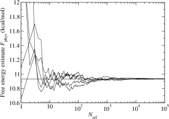
Figure 2: Absolute free energy for methane estimated by the reference system method as a function of the number of reference structures $N_{\rm ref}$ used in the estimate. The solid horizontal line is the exact free energy obtained by numerical integration. Five independent simulations are shown on a log scale to clearly show the convergence of the free energy estimate. Results shown were obtained using Eq. (10) with one-hundred bins for each degree of freedom, i.e., the estimates for the absolute free energy of methane in Table 1 are the values shown here for $N_{\rm ref}=1,000,000$.

Figure 2 shows the convergence behavior of the reference system method for methane. Five independent absolute free energy estimates are shown as a function of the number of reference structures used in the estimate. Each of the five simulations use the same protocol as described above, i.e., the absolute free energy estimates in Table 1 are the values shown in Fig. 2 for $N_{\rm ref}=100,000$.

Methane was chosen as a test system because intra-molecular interactions are due only to bond lengths and angles. In the OPLS-AA forcefield no non-bonded terms are present in the potential energy $U_{\rm phys}$, and thus the exact absolute free energy can be computed numerically without great difficulty. For methane, a configuration is determined by: (i) four bond lengths, which are independent of each other and all of other coordinates in the forcefield; and (ii) five bond angles which are correlated to one another but not to the bond lengths. Thus the exact partition function $Z_{\rm meth}$ is a product of four bond length partition functions $Z_{r}$ and one angular partition function $Z_{\theta}$,

$$Z_{\rm meth}=Z_{r}^{4}Z_{\theta},$$

$$Z_{r}=\int_{0}^{\infty}dr\;e^{-\beta U_{\rm phys}(r)},$$

$$Z_{\theta}=\int_{0}^{\pi}d\theta_{1}d\theta_{2}d\theta_{3}d\theta_{4}d\theta_{5}\;e^{-\beta U_{\rm phys}(\theta_{1},\theta_{2},\theta_{3},\theta_{4},\theta_{5})}.$$ (13)

$U_{\rm phys}(r)$ is harmonic and thus $Z_{r}$ was computed analytically using parameters from the forcefield. For $U_{\rm phys}(\theta_{1},\theta_{2},\theta_{3},\theta_{4},\theta_{5})$ the correlations between angles must be taken into account, thus $Z_{\theta}$ was estimated numerically using TINKER to evaluate $U_{\rm phys}$ in the five-dimensional integral. We found that $F_{\rm meth}=-k_{B}T\ln Z_{\rm meth}=10.932$ kcal/mol as shown in Table 1.

Methane was also used to show that the method correctly computes the free energy even when the physical ensemble is incorrect or incomplete. In our studies we found that the correct free energy is obtained using our method even when the histogram for each coordinate was assumed to be flat, i.e., without the use of a physical ensemble (data not shown).

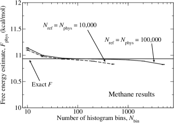
Figure 3: Absolute free energy for methane estimated by the reference system method as a function of the number of histogram bins used for each degree of freedom. The plot shows the “sweet spot” where histogram bins are small enough to reveal histogram features, yet large enough to give sufficient population in each bin. The results are shown with a vertical scale of two kcal/mol and on a log scale to emphasize the wide range of bin sizes that produce excellent results for the reference system approach. Results shown were obtained using Eq. (10) for a methane molecule using $N_{\rm phys}=N_{\rm ref}=10,000$ (dashed curve) and $N_{\rm phys}=N_{\rm ref}=100,000$ (solid curve). The solid horizontal line shows the exact free energy and the errorbars are the standard deviations of five independent trials. The plot demonstrates at least fifty bins should be used for each independent coordinate, and that the maximum number of bins depends on the number of snapshots in the physical ensemble.

Choosing the size of the histogram bins is an important consideration. Figure 3 shows the large “sweet spot” where bins are large enough to be well populated, and yet small enough to reveal histogram features. The figure shows results for the absolute free energy for a methane molecule using ten-thousand structures in both the physical and reference ensembles, $N_{\rm phys}=N_{\rm ref}=10,000$, (dashed curve) and $N_{\rm phys}=N_{\rm ref}=100,000$ (solid curve). The small vertical scale of two kcal/mol and the logarithmic horizontal scale emphasize that there is a wide range of bin sizes that produce excellent results for the reference system approach. Error bars are the standard deviation of five independent simulations. The solid horizontal line shows the exact free energy and the curves are free energy estimates, using Eq.  (10) as a function of the number of bins used for the histograms for all degrees of freedom. From this plot it is clear that one should choose at least fifty bins, and that the maximum number of bins that should be used depends on the number of snapshots in the physical ensemble—more snapshots in the physical ensemble means one can use more bins for the reference system.

System	Estimate (kcal/mol)	Independent Estimate
$F_{\rm alpha}$	87.3 (0.7)	—
$F_{\rm beta}$	86.3 (0.7)	—
$\Delta F_{\rm alpha\rightarrow beta}$	-1.0 (0.9)	-0.85 (0.05)

Table 2: Absolute free energy estimates of the alpha ($F_{\rm alpha}$) and beta ($F_{\rm beta}$) conformations obtained using the reference system method for leucine dipeptide with GBSA solvation, in units of kcal/mol. The independent measurement for the free energy difference was obtained via a 1.0 $\mu$s unconstrained simulation. The uncertainty for the absolute free energies, shown in parentheses, is the standard deviation from five independent 10.0 ns leucine dipeptide simulations using one-million reference structures in the reference ensemble. The uncertainty for the free energy differences is obtained by using every possible combination of $F_{\rm alpha}$ and $F_{\rm beta}$, i.e., twenty-five independent estimates. The standard error associated with the $\Delta F_{\rm alpha\rightarrow beta}$ reference system estimate is 0.18 kcal/mol, reflecting the twenty-five independent estimates. The table shows estimates of the configurational integral in Eq. (2), i.e., the constant term is not included in the estimate.

III.2 Leucine dipeptide

Table 2 shows the agreement for leucine dipeptide (ACE-(leu)₂-NME) between the free energy difference $\Delta F_{\rm alpha\rightarrow beta}$ as predicted by the reference system method, and as predicted via long simulation. The leucine dipeptide physical ensembles were generated using TINKER 4.2 tinker with the OPLS-AA forcefield. oplsaa The temperature was maintained at 500.0 K (to enable an independent $\Delta F$ estimate via repeated crossing of the free energy barrier between alpha and beta configurations), using Langevin dynamics with a friction coefficient of 5.0 ${\rm ps}^{-1}$. GBSA still implicit solvation was used, and RATTLE was utilized to maintain all bonds involving hydrogens at their ideal lengths rattle allowing the use of a 2.0 fs time step.

We calculated reference systems and computed absolute free energies of the alpha and beta conformations based on five 10.0 ns trajectories. For all simulations, backbone torsions were constrained using a flat-bottomed harmonic restraint (zero force if the torsion angles were within the allowed range, and harmonic otherwise), namely, for alpha: $-105<\phi<-45\;{\rm and}\;-70<\psi<-10$; and for beta: $-125<\phi<-65\;{\rm and}\;120<\psi<180$. The reference system was generated using 100,000 snapshots from the physical ensemble, then free energy estimates were obtained by generating 1,000,000 structures for the reference ensemble for each estimate. All one-hundred fifteen (excludes bond lengths constrained by RATTLE rattle) internal coordinates were binned as independent with fifty bins for each coordinate. The uncertainty shown in parenthesis is the standard deviation from the five independent estimates using the five separate trajectories, i.e., five different physical ensembles and five different reference systems.

Since independent estimates of the absolute free energies of the alpha and beta conformations of leucine dipeptide are not available, we calculated the free energy difference $\Delta F_{\rm alpha\rightarrow beta}=-0.85\;(0.05)$ kcal/mol via a 1.0 $\mu$s unconstrained simulation. The uncertainty of the independent estimate was obtained using block averages. The temperature was chosen to be 500.0 K which allowed around 1500 crossings of the free energy barrier between the alpha and beta conformations, providing an accurate independent estimate. As can be seen in Table 2, our estimated free energy difference is in good agreement with the independent value obtained via long simulation.

We emphasize that the nearly kcal/mol fluctuations observed in our leucine dipeptide estimates are completely independent of the magnitude of the free energy difference of the same order. That is, for a similar sized system and similar CPU investment, one would expect similar uncertainty, even for a very large free energy difference. This, indeed, is the motivation for performing absolute free energy calculations. We believe, moreover, that efficiency improvements will be achieved beyond the data in this initial report.

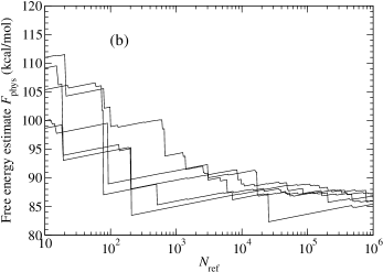
Figure 4: Free energy for leucine dipeptide estimated by the reference system method as a function of the number of reference structures $N_{\rm ref}$ used in the estimate. Five independent simulations are shown on a log scale to demonstrate the convergence behavior of the free energy estimate for (a) the alpha configuration, and (b) the beta configuration. Results shown were obtained using Eq. (10) with fifty bins for each degree of freedom.

Figure 4 shows the convergence behavior of the reference system method for leucine dipeptide. Five free energy estimates are shown as a function of the number of reference structures used in the estimate for (a) the alpha configuration, and (b) the beta configuration. Each of the five simulations use the same protocol as described above.

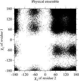
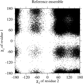
Figure 5: Scatter plots of the two $\chi_{2}$ torsions of each residue for leucine dipeptide. Results are shown for both physical and reference ensembles containing 100,000 structures each. The figure shows that: (i) the reference system has good overlap with the physical system, as can be seen by the similarity between the two plots; and (ii) the reference system is more broadly distributed than the physical system, as evidenced by the data at (-60,-60) for the reference system that is not present for the physical system.

The leucine dipeptide calculations also demonstrate two important aspects of the particular reference system defined in this study: (i) the reference system has good overlap with the physical system; and (ii) the reference system is broader than the physical system. Figure 5 shows a scatter plot of the $\chi_{2}$ torsions of each residue for both the physical and reference ensembles. Each ensemble contains 100,000 structures. The figure clearly shows the excellent overlap between the reference and physical ensemble, as can be seen by the similarity between the two plots. In addition, the reference ensemble scatter plot has data in the region (-60,-60) which does not exist in the physical ensemble, showing that the reference system is “broader” than the physical system.

Figure 6: Histogram of the distance between the $C_{\delta}$ of residue one and the $C_{\alpha}$ of residue two for leucine dipeptide. Results are shown for both reference and physical ensembles containing 100,000 structures each. The figure shows that: (i) the reference system has good overlap with the physical system; and (ii) the reference system is broader than the physical system.

Figure 6 shows a histogram of the distance between the $C_{\delta}$ atom of residue one and the $C_{\alpha}$ of residue two for the same ensembles as Fig. 5. The figure again shows how the reference system has both excellent overlap with the physical system and is also broader than the physical system.

IV Discussion

The present results raise a number of questions regarding the reference system approach to computing absolute free energies—in particular, regarding the use of correlations, the importance of the physical ensemble, and the potential for application to larger systems.

IV.1 Correlation of Coordinates

How can correlations among coordinates be used to increase the method’s effectiveness? One may choose to bin coordinates as independent (i.e., one-dimensional histograms), or with correlations (i.e., multi-dimensional histograms). For example, in peptides, one may choose to bin all sets of backbone $\phi,\psi$ torsions as correlated, and all other coordinates (bond lengths, bond angles, other torsions) as independent. It might always seem advantageous to bin some coordinates (at least backbone torsions) as correlated, since reference structures drawn randomly from the histograms will be less likely to have steric clashes. On the other hand, including correlations with small bin sizes is impractical. As an example, imagine that for the leucine dipeptide molecule used in this study, one binned the four $\phi,\psi$ backbone torsions as correlated. If fifty bins for each torsion were used (as should be done according to the discussion below), then there would be $50^{4}=6,250,000$ multi-dimensional bins to populate, which is simply not feasible.

There does appear to be an important advantage to eliminating at least some correlations from the original “physical” ensemble: namely, a larger portion of conformational space becomes available to the reference ensemble; see Figs. 5 and 6. Since coordinates for the reference structures are drawn randomly and independently, it is possible to generate reference structures that are in entirely different energy basins than those in the physical ensemble. It is thus possible to overcome the inadequacies of the physical ensemble by binning internal coordinates independently. The optimal (presumably) limited use of correlations will be considered in future work.

Regardless of the degree of correlations included in $U_{\rm ref}$, we emphasize that final results fully include correlations in the physical potential $U_{\rm phys}$.

IV.2 Quality of the physical ensemble

Since the reference ensemble is generated by drawing at random from histograms which, in turn, were generated from the physical ensemble, a natural question to ask is: how complete does the physical ensemble need to be? The surprising answer is that, for our reference system method, the physical ensemble does not need to be complete, or even correct (properly distributed). Since Eqs. (3) and (9) are valid for arbitrary reference systems, the convergence of the free energy estimate to the correct value is guaranteed, in the limit of infinite sampling ($N_{\rm ref}\rightarrow\infty$), regardless of the quality of the physical ensemble. The “trick” is that the ensemble for the reference system must be converged, which can be achieved with much less expense since there is no dynamical trapping. Unlike the typical case for molecular mechanics simulation, we sample the reference ensemble “perfectly”—there is no possibility of being trapped in a local basin. By construction, since all coordinate values are generated exactly according to the reference distributions, the reference ensemble can only suffer from statistical (but not systematic) error. For example, it was possible to obtain the correct free energy for methane based on 10,000 reference structures even when the histogram for each coordinate was assumed to be flat, i.e., without the use of a physical ensemble (data not shown).

It is important to note that, while convergence to the correct free energy is guaranteed for any choice of reference system, the efficiency of the method could be dramatically reduced if the reference system does not overlap well with the physical system.

Given the fact that the physical ensemble need not be correct, it is easy to imagine a modified method that does not require simulation, but instead populates the histogram bins using the “bare” potential for each internal coordinate (e.g., Gaussian histograms for bond lengths and angles). Of course, the conformational state must be defined explicitly, with upper and lower limits for coordinates. Allowed ranges for the torsions (especially $\phi,\psi$) are naturally obtainable via, e.g., Ramachandran propensities (e.g., Ref. richardson), and reasonable ranges for bond lengths and angles could be chosen to be, e.g., several standard deviations from the mean.

IV.3 Extension to larger systems

While the initial results of our reference system method are promising, a naive implementation of the method will find difficulty with large systems (as do all absolute and relative free energy methods). For our method, the difficulty with including a very large number of degrees of freedom is due to the fact that, if one does not treat all correlations in the backbone, then steric clashes will occur frequently when generating the reference ensemble.

However, it is possible to extend the method to larger peptides, still include all degrees of freedom, and bin all coordinates independently (important for broadening configurational space, as discussed above), by using a “segmentation” technique motivated by earlier work. gibson-seg; leach-seg Consider generating reference structures for a ten-residue peptide in the alpha helix conformation. Due to the large number of backbone torsions, most of the reference structures chosen at random will not be energetically favorable. However, if one breaks the peptide into two pieces, then one can generate many structures for each segment, and only “keep” energetically likely segment structures. The selected structures may be joined to form full structures which are reasonably likely to have low energy. For example, if one generates $10^{5}$ structures for each of the two segments and keeps only $10^{3}$ of those, then one only need evaluate $10^{3}\times 10^{3}=10^{6}$ full structures out of a possible $10^{5}\times 10^{5}=10^{10}$. A statistically correct segmentation strategy is currently being investigated by the authors for use in large peptides.

Another strategy which may prove useful for larger systems is to use the reference system method with multi-stage simulation. Multi-stage simulation requires the introduction of a hybrid potential energy parameterized by $\lambda$, e.g.,

$$U_{\lambda}=\lambda U_{\rm phys}+(1-\lambda)U_{\rm ref}.$$ (14)

Thus, $U_{0}=U_{\rm ref}$ and $U_{1}=U_{\rm phys}$. Simulations are performed using the hybrid potential energy $U_{\lambda}$ (and thus a hybrid forcefield, if using molecular dynamics) at intermediate $\lambda$ values between 0 and 1. Conventional free energy methods such as thermodynamic integration or free energy perturbation can then be used to obtain $F_{\rm phys}$.

We also believe that including correlations, such as suggested by Eq. (6) and possibly other ways, may be useful. The inclusion of correlations should improve the overlap between the reference and physical ensembles—thereby reducing the amount of sampling required in the reference system, hence improving efficiency. This also will be explored in future work. (We also remind the reader that the final free energy value includes the full correlations in $U_{\rm phys}$, regardless of $U_{\rm ref}$.)

The method could prove useful in future protein-ligand binding studies. In the simplest approach, one could freeze all degrees of freedom except for the ligand and side-chain degrees of freedom in the binding site. While the absolute free energy would be unphysical, the approach could permit comparison of ligands or protein mutations with little or no conformational similarity.

In principle, it is possible to extend the reference system method to include explicitly solvated biomolecules. However, as with all absolute free energy methods, the addition of the solvent degrees of freedom causes the free energy estimate to converge much more slowly than without explicit solvent. Thus, we feel the method described in this study will find use primarily in implicitly solvated biomolecules.

V Conclusions

In conclusion, we have introduced and tested a simple method for calculating absolute free energies in molecular systems. The approach relies on the construction of an ensemble of reference structures (i.e., the reference system) that is designed to have high overlap with the physical system of interest. The method was first shown to reproduce exactly computable absolute free energies for simple systems, and then used to correctly predict the stability of leucine dipeptide conformations using all one-hundred fifteen degrees of freedom.

Some strengths of the approach are that: (i) the reference system is built to have good overlap with the system of interest by using internal coordinates and by using a single equilibrium ensemble from Monte Carlo or molecular dynamics; (ii) the absolute free energy estimate is guaranteed to converge to the correct value, whether or not the physical ensemble is complete and, in fact, it is possible to estimate the absolute free energy without the use of a physical ensemble; (iii) the method explicitly includes all degrees of freedom employed in the simulation; (iv) the reference system need only be numerically computable, i.e., the exact analytic result is not needed; and (v) the method can be trivially extended to include the use of multi-stage simulation. The CPU cost of the approach, beyond that for short trajectories of the physical system of interest, is one energy call for each reference structure, plus the less expensive cost of generating the reference ensemble.

In the present “proof of principle” report, our method was used to study conformational equilibria; however we feel that the simplicity and flexibility of the method may find broad use in computational biophysics and biochemistry for a wide variety of free energy problems. We have also described a segmentation strategy, currently being pursued, to use the approach in much larger systems.