Test of the isotropy of the speed of light using a continuously rotating optical resonator

Abstract

We report on a test of Lorentz invariance performed by comparing the resonance frequencies of one stationary optical resonator and one continuously rotating on a precision air bearing turntable. Special attention is paid to the control of rotation induced systematic effects. Within the photon sector of the Standard Model Extension, we obtain improved limits on combinations of 8 parameters at a level of a few parts in $10^{-16}$. For the previously least well known parameter we find $\tilde{\kappa}_{e-}^{ZZ}=(-1.9\pm 5.2)\times 10^{-15}$. Within the Robertson-Mansouri-Sexl test theory, our measurement restricts the isotropy violation parameter $\beta-\delta-\frac{1}{2}$ to $(-2.1\pm 1.9)\times 10^{-10}$, corresponding to an eightfold improvement with respect to previous non-rotating measurements.

Local Lorentz invariance (LLI) is an essential ingredient of both the standard model of particle physics and the theory of general relativity. It states that locally physical laws are identical in all inertial reference frames i.e. independent of velocity and orientation. However, several attempts to formulate a unifying theory of quantum gravity discuss tiny violations of LLI. Modern high precision test experiments for LLI are considered as important contributions to these attempts, as they might either rule out or possibly reveal the presence of such effects at some level of measurement precision. An experiment of particular sensitivity to LLI-violation is the Michelson-Morley (MM) experiment MM testing the isotropy of the speed of light. Modern versions employ high finesse electromagnetic resonators, whose eigenfrequencies depend on the speed of light $c$ in a geometry dependent way ($\nu\sim c/L$ for a linear optical Fabry-Perot cavity of length $L$). Thus a measurement of the eigenfrequency of a resonator as its orientation is varied, should reveal an anisotropy of $c/L$.
Recently, such an anisotropy of $c$ has been described as a consequence of broken Lorentz symmetry within a test model called Standard Model Extension (SME) Kost02 . This model adds all LLI violating terms that can be formed from the known fields and Lorentz tensors to the Lagrangian of each sector of the standard model of particle physics. It thus allows a consistent and comparative analysis of various experimental tests, including the MM experiment. The latter however, is also often interpreted according to a kinematical test theory, formulated by Robertson Robertson and Mansouri and Sexl MS (RMS). This test theory assumes a preferred frame, commonly adopted to be the cosmic microwave background (CMB). Combinations of three test parameters ($\alpha$, $\beta$, $\delta$) then model an anisotropy as well as a boost dependence of $c$ within a frame moving at velocity $v$ relative to the CMB.
In view of the substantial impact that LLI-violation would have all over physics, the new approach of the SME has triggered a new generation of improved MM-type experiments MMPRL ; Wolf ; WolfPRD ; Lipa . So far all of these recent measurements relied solely on Earth’s rotation for varying resonator orientation, which was made possible by the low drift properties of cryogenically cooled resonators. However, actively rotating the setup as done in a classic experiment by Brillet and Hall BrilletHall offers two strong benefits: (i) the rotation rate can be matched to the timescale of optimal resonator frequency stability and (ii) the statistics can be significantly improved by performing thousands of rotations per day. While otherwise using equipment similar to that in the non rotating experiments, these advantages should allow for tests improved by orders of magnitude – assuming that systematic effects induced by the active rotation can be kept sufficiently low.

Here we present the first implementation of such a continuously rotating optical MM-type experiment since BrilletHall . Concurrent work of other groups, however, also features similar experiments either using continuously rotating microwave cavities Stanwix or cryogenic optical resonators, whose orientation is periodically changed by $90^{\circ}$ Schiller . At the core of the experimental setup is an optical cavity fabricated from fused silica (L = 3 cm, 20 kHz linewidth) which is continuously rotated on a precision air bearing turntable. Its frequency is compared to that of a stationary cavity oriented north-south (L = 10 cm, 10 kHz linewidth). Each cavity is mounted inside a thermally shielded vacuum chamber. The cavity resonance frequencies are interrogated by two diode pumped Nd:YAG lasers (1064 nm), coupled to the cavities through windows in the vacuum chambers, and stabilized to cavity eigenfrequencies using the Pound-Drever-Hall method Dre83 . The table rotation rate $\omega_{\rm rot}=2\pi/T$ is set to $T$ $\sim$ 43 s ($\sim$ 2000 rotations/day) matching the time scale of optimum cavity stability ($\Delta\nu/\nu=1\times 10^{-14}$). At this rotation rate it is also possible to rely on the excellent thermal isolation properties of the vacuum chambers at room temperature (time constant $\sim 10$ h). The residual temperature drift of the resonance frequencies is on the order of 1 MHz/day, which is comparatively high but sufficiently linear to be cleanly separated from a potential LLI-violation signal at $2\omega_{\rm{rot}}$.
Fig.1 gives a schematic view of the rotating setup. Electrical connections are made via an electric 15 contact slip ring assembly on top. To measure the frequency difference $\Delta\nu$ of both lasers, a fraction of the rotating laser’s light leaves the table aligned with the rotation axis (see Fig.1) and is then overlapped with light from the stationary laser on a high speed photodetector. The resulting beat note at the difference frequency $\Delta\nu\sim$2 GHz is read out at a sampling rate of 1/s after down conversion to about 100 MHz.

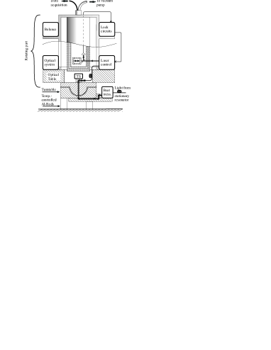
Figure 1: Setup of the rotating part of the experiment. A high performance turntable is applied specified for rotation axis wobble $<1\mu$rad. The center-of-mass of the setup is carefully balanced and tilt is monitored using an electronic bubble level tilt sensor (TS).

We expended substantial effort on minimizing systematic effects associated with turntable rotation (see Fig.2). In addition to good thermal and electromagnetic shielding, this most importantly involves limiting cavity deformations due to external forces (gravitational and centrifugal). If the cavity is not supported in a perfectly symmetric manner, its frequency is particularly susceptible to tilt. We observe a relative frequency change of $1.5\times 10^{-16}/\mu$rad. As tilts which vary as a function of the orientation of the turntable enter the analysis of the experiment, such changes have to be suppressed by keeping the rotation axis as vertical as possible and preventing wobble in the setup. The latter is achieved by employing a turntable with intrinsic wobble $<1$ $\mu$rad and carefully balancing the center-of-mass of the rotating part. To prevent long term variations of rotation axis tilt, an active tilt control is applied. Similar to the scheme described by J. Gundlach Gundlach , we place the table on three aluminum cylinders, $20$ cm in length, two of which can be heated independently in order to use thermal expansion ($5\mu$m/${}^{\circ}C$) to compensate slow tilt variations. The heating is part of a computer controlled closed servo loop, and the tilt is monitored using an electronic bubble level sensor of 0.1 $\mu$rad resolution placed at the turntable center. Typical tilt variations of the laboratory’s ground floor are several 10 $\mu$rad/day. Without tilt control these would give rise to (varying) systematic effects at $2\omega_{\rm{rot}}$ of up to one part in $10^{-14}$. The active stabilization reduces tilt variations to $<1\mu$rad corresponding to systematic tilt induced effects $<10^{-16}$.

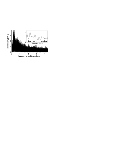
Figure 2: Fourier transform of a 4-day data set starting on February 18, 2005, with active tilt control applied (after removal of long term drift). Insert: No peak is visible at $2\omega_{\rm rot}$ nor at the siderial sidebands.

For our setup, the fundamental signal indicating an anisotropy due to a LLI-violation is a sinusoidal variation of the beat frequency at $2\omega_{\rm{rot}}$. As described in Kost02 the amplitude of this signal in turn is expected to be modulated due to Earth’s rotation at $\omega_{\oplus}$ (and at Earth’s orbital motion $\Omega_{\oplus}$, which will be considered below). This can be expressed as

$$\frac{\Delta\nu}{\nu_{0}}=S(t)\sin 2\omega_{\rm rot}t+C(t)\cos 2\omega_{\rm rot}t,$$ (1)

where $\nu_{0}\sim 2.82\times 10^{14}$ Hz is the undisturbed laser frequency and the amplitudes $S(t)$ and $C(t)$ vary according to

$$S(t) = S_{0}+S_{s1}\sin\omega_{\oplus}t+S_{c1}\cos\omega_{\oplus}t+$$

$$S_{s2}\sin 2\omega_{\oplus}t+S_{c2}\cos 2\omega_{\oplus}t,$$

$$C(t) = C_{0}+C_{s1}\sin\omega_{\oplus}t+C_{c1}\cos\omega_{\oplus}t+$$

$$C_{s2}\sin 2\omega_{\oplus}t+C_{c2}\cos 2\omega_{\oplus}t.$$

From each continuous measurement of $\Delta\nu$ comprising 2000 to 10000 rotations, we determine the set of ten Fourier coefficients $\{S_{i},C_{i}\}$ within Eq.(Test of the isotropy of the speed of light using a continuously rotating optical resonator) and Eq.(Test of the isotropy of the speed of light using a continuously rotating optical resonator) in a similar way as in Schiller . To minimize cross-contamination between Fourier coefficients we only consider data windows that are integer multiples of 24 hours in length. This method was carefully validated by analyzing test data sets created by superimposing a hypothetical violation signal to our data, and checking that the known Fourier coefficients were reliably reproduced. The procedure is as follows: We divide the data into subsets of 10 table rotations each (200 subsets/24 h) and use a least squares fit to Eq.(1) for each subset phase . To obtain a proper fit in the presence of drift and small residual systematics at $\omega_{\rm{rot}}$, we include additional sine and cosine components at $\omega_{\rm{rot}}$, an offset, and a linear and quadratic drift. At the chosen subset size this is sufficient to cleanly separate the frequency drift from the signal at $2\omega_{\rm{rot}}$. Next, we fit the resulting distributions of $S(t)$ and $C(t)$ with Eq.(Test of the isotropy of the speed of light using a continuously rotating optical resonator) and Eq.(Test of the isotropy of the speed of light using a continuously rotating optical resonator) phase yielding the complete set $\{S_{i},C_{i}\}$ and individual fit errors for each coefficient.
Following this scheme we analyzed 15 data sets of 24 h to 100 h in length, spanning December 2004 to April 2005 and comprising $\sim 70000$ turntable rotations in total. Fig.3 shows the resulting Fourier coefficients $\{S_{i},C_{i}\}$ as a function of time together with their weighted average values. Note that a small systematic effect at $2\omega_{\rm rot}$ is still present affecting the components $C_{0}$ and $S_{0}$ in particular. This has to be specially considered within the interpretation of these results according to the two test theories SME and RMS given below.

Table 1: Left column: Fourier components $C_{i}$ related to the SME parameters for short measurements $\ll 1$ year. These relations are obtained according to the calculation in Kost02 and adopting $\chi=37.5^{\circ}$ as the laboratory colatitude. $\phi=\Omega_{\oplus}t$ is the siderial phase relative to t = 0 when the Earth passes vernal equinox.
Right column: $C_{i}$ related to the RMS-parameter B. $v$ is the velocity of the laboratory relative to the CMB (neglecting Earth’s orbital and rotational boost here). $\alpha=168^{\circ}$ and $\gamma=-6^{\circ}$ fix the orientation of v in the sun centered reference frame. The respective $S_{i}$ amplitudes are related according to $S_{0}=0$, $S_{s1}=-C_{c1}/\cos\chi$, $S_{c1}=C_{s1}/\cos\chi$, $S_{s2}=-2C_{c2}\cos\chi/(1+\cos^{2}\chi)$, $S_{c2}=2C_{s2}\cos\chi/(1+\cos^{2}\chi)$.

	SME	RMS
$C_{0}$	$0.14\tilde{\kappa}_{e-}^{ZZ}-7.4\times 10^{-6}\tilde{\kappa}_{o+}^{XY}\cos\phi-8.5\times 10^{-6}\tilde{\kappa}_{o+}^{XZ}\cos\phi-9.3\times 10^{-6}\tilde{\kappa}_{o+}^{YZ}\sin\phi$	$\frac{1}{8}(-1+3\cos 2\gamma)\sin^{2}\chi\frac{v^{2}}{c^{2}}B$
$C_{s1}$	$-0.24\tilde{\kappa}_{e-}^{YZ}+2.2\times 10^{-5}\tilde{\kappa}_{o+}^{XY}\cos\phi-9.6\times 10^{-6}\tilde{\kappa}_{o+}^{XZ}\cos\phi$	$-\frac{1}{4}\sin\alpha\sin 2\gamma\sin 2\chi\frac{v^{2}}{c^{2}}B$
$C_{c1}$	$-0.24\tilde{\kappa}_{e-}^{XZ}-2.4\times 10^{-5}\tilde{\kappa}_{o+}^{XY}\sin\phi+9.6\times 10^{-6}\tilde{\kappa}_{o+}^{YZ}\cos\phi$	$-\frac{1}{4}\cos\alpha\sin 2\gamma\sin 2\chi\frac{v^{2}}{c^{2}}B$
$C_{s2}$	$0.41\tilde{\kappa}_{e-}^{XY}-4.1\times 10^{-5}\tilde{\kappa}_{o+}^{XZ}\sin\phi-3.7\times 10^{-5}\tilde{\kappa}_{o+}^{YZ}\cos\phi$	$-\frac{1}{4}\sin 2\alpha\cos^{2}\gamma(1+\cos^{2}\chi)\frac{v^{2}}{c^{2}}B$
$C_{c2}$	$0.2[\tilde{\kappa}_{e-}^{XX}-\tilde{\kappa}_{e-}^{YY}]-3.7\times 10^{-5}\tilde{\kappa}_{o+}^{XZ}\cos\phi+4.1\times 10^{-5}\tilde{\kappa}_{o+}^{YZ}\sin\phi$	$-\frac{1}{4}\cos 2\alpha\cos^{2}\gamma(1+\cos^{2}\chi)\frac{v^{2}}{c^{2}}B$

For the photonic sector of the SME the LLI violating extension contains 19 independent parameters, which can be arranged into one scalar $\kappa_{tr}$, and four traceless $3\times 3$ matrices: $\tilde{\kappa}_{e-}$, $\tilde{\kappa}_{o+}$, $\tilde{\kappa}_{e+}$ and $\tilde{\kappa}_{o-}$. While $\kappa_{tr}$ is related to the one way speed of light Tobar , the elements of the latter two matrices are restricted to values $<10^{-32}$ by astrophysical observations Kost01 . The remaining matrices $\tilde{\kappa}_{e-}$ and $\tilde{\kappa}_{o+}$ contain 8 parameters that describe a boost dependent ($\tilde{\kappa}_{o+}$, antisymmetric) and a boost independent ($\tilde{\kappa}_{e-}$, symmetric) anisotropy of the speed of light. Recent measurements have restricted 7 of these elements to a level of $10^{-11}$ respectively $10^{-15}$ MMPRL ; Wolf ; WolfPRD ; Lipa . $\tilde{\kappa}_{e-}^{ZZ}$ can only be determined in actively rotating experiments thus it was not accessible in these experiments, as they relied solely on Earth’s rotation.
The dependence of the determined Fourier coefficients on these SME parameters, referred to a Sun centered coordinate system, can be calculated as outlined in Kost02 . To first order in orbital boosts we obtain the combinations given in Tab.1. The amplitudes contain siderial phase factors, that account for a modulation of the boost dependent $\tilde{\kappa}_{o+}$ terms due to Earth’s orbit. For data sets spanning $>1$  year this allows the independent determination of $\kappa_{o+}$ and $\kappa_{e-}$ terms by fitting these variations to the respective distributions of coefficients $\{S_{i},C_{i}\}$. However, as our data currently only spans 4 months, we can only extract limits on individual parameters if we additionally assume no cancellation between the $\tilde{\kappa}_{e-}$ terms and $\tilde{\kappa}_{o+}$ terms. Based on this assumption we obtain the values given in Tab. 2. These limits on the order of few parts in $10^{-16}$ improve the ones obtained in WolfPRD by up to a factor of eight. A future analysis including data covering a longer time period will be able to remove the assumption of non-cancellation.

Table 2: SME parameters extracted from a fit of the relations of Tab.1 to the respective distributions of Fourier components $\{S_{i},C_{i}\}$ as shown in Fig.3. Note that these limits are based on the assumption of no cancellation between $\tilde{\kappa}_{e-}$ and varying $\tilde{\kappa}_{o+}$ terms. All $\tilde{\kappa}_{e-}$ values are $\times 10^{-16}$, $\tilde{\kappa}_{o+}$ values are $\times 10^{-12}$.

index	$ZZ$	$XX-YY$	$XY$	$XZ$	$YZ$
$\tilde{\kappa}_{e-}$	-19.4 (51.8)	5.4 (4.8)	-3.1 (2.5)	5.7 (4.9)	-1.5 (4.4)
$\tilde{\kappa}_{o+}$	-	-	-2.5 (5.1)	-3.6 (2.7)	2.9 (2.8)

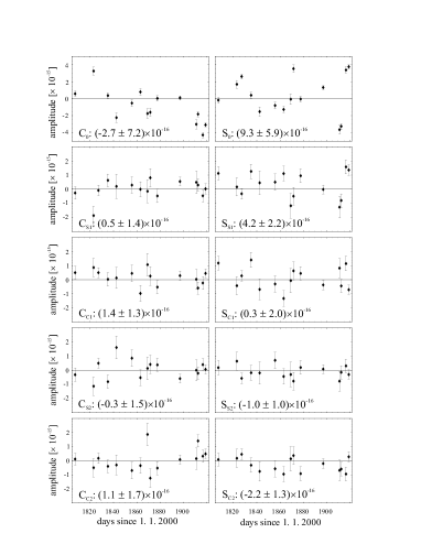
Figure 3: Each graph gives the distribution of a certain Fourier coefficient of Eq.(Test of the isotropy of the speed of light using a continuously rotating optical resonator) and Eq.(Test of the isotropy of the speed of light using a continuously rotating optical resonator) in time. Note the different scale for $C_{0}$ and $S_{0}$ affected by small systematic effects. The time axis spans December 2004 to April 2005. 15 points are included in total, each point is determined from one continuous data set comprising 2000 - 10000 rotations. Within each graph the weighted average value of the respective coefficient is given.

The parameter $\tilde{\kappa}_{e-}^{ZZ}$ needs a special consideration as it only enters $C_{0}$, and might thus be compromised by the systematic effects. However, we observe that the phase of this residual systematic signal varies widely between individual measurements. The systematic effect thus averages out resulting only in an increased error bar on the mean value of this component. As the systematic effects are comparatively small, we can still improve the limit on $\tilde{\kappa}_{e-}^{ZZ}$ set by Stanwix . From the average value of $C_{0}$ we deduce a limit for $(\tilde{\kappa}_{e-})^{ZZ}$ of $(-1.9\pm 5.2)\times 10^{-15}$, taking into account that the contributions to $C_{0}$ from the $\tilde{\kappa}_{o+}$-terms are already restricted to $<10^{-15}$ by the other Fourier components. While $(\tilde{\kappa}_{e-})^{ZZ}$ plays no special role among the components of the $\tilde{\kappa}_{e-}$-matrix, setting such stringent limits on it is especially important from an experimental point of view, as it most directly indicates our ability to control rotation related systematic effects.
For comparison to earlier work we also give an analysis within the RMS framework. This test theory models an anisotropy of the speed of light according to $\Delta c\sim B\frac{v^{2}}{c^{2}}\sin^{2}\theta$, where $B$ abbreviates the RMS test parameter combination $(\beta-\delta-\frac{1}{2})$. $v$ is the laboratory velocity relative to the CMB and $\vartheta$ is the angle between direction of light propagation and $v$. $B$ enters the $\{S_{i}$,$C_{i}\}$ Fourier amplitudes as shown in Tab.1 if we neglect modulation of $v=370$ km/s due to orbital boosts. To determine B from our data we simultaneously fit these functions to the respective distributions of Fourier coefficients in Fig. 3, excluding $C_{0}$ compromised by systematic effects. This results in $B=(-2.1\pm 1.9)\cdot 10^{-10}$, which is a factor of eight improvement in accuracy compared to the non rotating experiment of MMPRL .

In conclusion, our setup applying precision tilt control proves that comparatively high rotation rate can be achieved at low systematic disturbances. This lifts a severe limitation from actively rotated MM-type experiments as performed in the past BrilletHall , and provides the possibility to increase sensitivity of these tests to LLI-violation by orders of magnitude. At the current status of our measurement we can already set limits on several test theory parameters that are more stringent by up to a factor of eight. An extended analysis of the experiment within the SME shows that it is also sensitive to parameters from the electronic sector of the SME that change the cavity length MuePRD . While this provides the possibility to set limits on further SME parameters, we leave it for a future analysis. The main limitation of accuracy within our experimental setup currently arises from laser lock stability. Thus, the implementation of an active vibration isolation as well as new cavities is underway, which should enable us to improve laser lock stability by about an order of magnitude.
We thank Claus Lämmerzahl for discussions and Jürgen Mlynek and Gerhard Ertl for making this experiment possible. S. Herrmann acknowledges support from the Studienstiftung des deutschen Volkes.

References

- (1) A.A. Michelson and E.W. Morley, Am. J. Sci 34, 333 (1887).
- (2) V.A. Kostelecký and M. Mewes, Phys. Rev. D 66, 056005 (2002).
- (3) H.P. Robertson, Rev. Mod. Phys. 21, 378 (1949).
- (4) R.M. Mansouri and R.U. Sexl , Gen. Rel. Gravit. 8, 497 (1977); see also C. Lämmerzahl et al., Int. J. Mod. Phys. D 11, 1109 (2002).
- (5) H. Müller et al., Phys. Rev. Lett. 91, 020401 (2003).
- (6) P. Wolf et al., Phys. Rev. Lett. 90, 060402 (2003).
- (7) P. Wolf et al., Phys. Rev. D 70, 051902(R) (2004).
- (8) J.A. Lipa et al., Phys. Rev. Lett. 90, 060403 (2003).
- (9) A. Brillet and J.L. Hall, Phys. Rev. Lett. 42, 549 (1979).
- (10) P.L. Stanwix et al., Phys. Rev. Lett. 95, 040404 (2005).
- (11) P. Antonini et al., Phys. Rev. A 71, 050101(R) (2005).
- (12) R.W.P. Drever et al., Appl. Phys. B 31, 97-105 (1983).
- (13) The phase of the respective fits is fixed by the test theory considered according to Kost02 .
- (14) J. Gundlach, priv. comm.; B.R. Heckel, Proc. of the Second Meeting on CPT and Lorentz Symmetry, Singapore: World Scientific, p173-180 (2002).
- (15) M.E. Tobar et al., Phys. Rev. D 71, 025004 (2005).
- (16) V.A. Kostelecký and M. Mewes, Phys. Rev. Lett. 87, 251304 (2001).
- (17) H. Müller et al., Phys. Rev. D 68, 116006 (2003); Phys. Rev. D 71, 045004 (2005).