Can one predict DNA Transcription Start Sites by studying bubbles?

Abstract

It has been speculated that bubble formation of several base-pairs due to thermal fluctuations is indicatory for biological active sites. Recent evidence, based on experiments and molecular dynamics (MD) simulations using the Peyrard-Bishop-Dauxois model, seems to point in this direction. However, sufficiently large bubbles appear only seldom which makes an accurate calculation difficult even for minimal models. In this letter, we introduce a new method that is orders of magnitude faster than MD. Using this method we show that the present evidence is unsubstantiated.

Double stranded DNA (dsDNA) is not a static entity. In solution, the bonds between bases on opposite strands can break even at room temperature. This can happen for entire regions of the dsDNA chain, which then form bubbles of several base-pairs (bp). These phenomena are important for biological processes such as replication and transcription. The local opening of the DNA double helix at the transcription start site (TSS) is a crucial step for the transcription of the genetic code. This opening is driven by proteins but the intrinsic fluctuations of DNA itself probably play an important role. The statistical and dynamical properties of these denaturation bubbles and their relation to biological functions have therefore been subject of many experimental and theoretical studies. It is known that the denaturation process of finite DNA chains is not simply determined by the fraction of strong (GC) or weak (AT) base-pairs. The sequence specific order is important. Special sequences can have a high opening rate despite a high fraction of GC base pairs Dornberger . For supercoiled DNA, it has been suggested that these sequences are related to places known to be important for initiating and regulating transcription PNAS1 . For dsDNA, Choi et al found evidence that the formation of bubbles is directly related the transcription sites ChoiNuc2004 . In particular, their results indicated that the TSS could be predicted on basis of the formation probabilities for bubbles of ten or more base-pairs in absence of proteins. Hence, the secret of the TSS is not in the protein that reads the code, but really a characteristics of DNA as expressed by the statement: DNA directs its own transcription ChoiNuc2004 . In that work, S1 nuclease cleavage experiments were compared with molecular dynamics (MD) simulations on the Peyrard-Bishop-Dauxois (PBD) model PB ; PBD of DNA. The method used is not without limitations. The S1 nuclease cleavage is related to opening, but many other complicated factors are involved. Moreover, theoretical and computational studies have to rely on simplified models and considerable computational power. As the formation of large bubbles occurs only seldom in a microscopic system, MD or Monte Carlo (MC) methods suffer from demanding computational efforts to obtain sufficient accuracy. Nevertheless, the probability profile found for bubbles of ten and higher showed a striking correlation with the experimental results yielding pronounced peaks at the TSS ChoiNuc2004 . Still, the large statistical uncertainties make this correlation questionable. To make the assessment absolute, we would either need extensively long or exceedingly many simulation runs or a different method that is significantly faster than MD.

In this letter, we introduce such a method for the calculation of bubble statistics for first neighbor interaction models like the PBD. We applied it to the sequences studied in Refs. ChoiNuc2004 and, to validate the method and to compare its efficiency, we repeated the MD simulations with 100 times longer runs. The new method shows results consistent with MD but with a lot higher accuracy than these considerably longer simulations. Armed with this novel method, we make a full analysis of preferential opening sites for bubbles of any length. This analysis shows that there is no strict analogy between these preferential sites and the TSS using equilibrium statistics. Hence, the previously found correlation must have been either accidental or due to some non-equilibrium effect, which remains speculative. We discuss this issue and, more generally, the required theoretical and experimental advancements that could address the title’s question definitely.

The PBD model reduces the myriad degrees of freedom of DNA to an one-dimensional chain of effective atom compounds describing the relative base-pair separations $y_{i}$ from the ground state positions. The total potential energy $U$ for an $N$ base-pair DNA chain is then given by $U(y^{N})=V_{1}(y_{1})+\sum_{i=2}^{N}V_{i}(y_{i})+W(y_{i},y_{i-1})$ with $y^{N}\equiv\{y_{i}\}$ the set of relative base pair positions and

$$V_{i}(y_{i}) = D_{i}\Big{(}e^{-a_{i}y_{i}}-1\Big{)}^{2}$$ (1)

$$W(y_{i},y_{i-1}) = \frac{1}{2}K\Big{(}1+\rho e^{-\alpha(y_{i}+y_{i-1})}\Big{)}(y_{i}-y_{i-1})^{2}$$

The first term $V_{i}$ is the on site Morse potential describing the hydrogen bond interaction between bases on opposite strands. $D_{i}$ and $a_{i}$ determine the depth and width of the Morse potential and are different for the AT and GC base-pair. The stacking potential $W$ consists of a harmonic and a nonlinear term. The second term was later introduced PBD and mimics the effect of decreasing overlap between $\pi$ electrons when one of two neighboring base move out of stack. As a result, the effective coupling constant of the stacking interaction drops from $K^{\prime}=K(1+\rho)$ down to $K^{\prime}=K$. It is due to this term that the observed sharp phase transition in denaturation experiments can be reproduced. All interactions with the solvent and the ions are effectively included in the force-field. The constants $K,\rho,\alpha,D_{\rm AT},D_{\rm GC},a_{\rm AT},a_{\rm GC}$ were parameterized in Ref. CAGI and tested on denaturation curves of short heterogeneous DNA segments. These examples show that, despite its simplified character, the model is able to give a quantitative description of DNA. Most importantly, it allows to study the statistical and dynamical behavior of very long heterogeneous DNA sequences, which is impossible for any atomistic model.

Despite these successes, it is important to realize the limitations of the model. The PBD model treats the A and T bases and the G and C bases as identical objects. The stacking interaction is also independent of the nature of the bases. Moreover, there is a subtle point that needs further explanation. As the PBD model basically represents a single dsDNA in an infinite solution, the probability for complete denaturation of a molecule of finite length, resulting in two single stranded DNAs, tends to unity with increasing time at any temperature. In the experiments, where the amount of solvated DNA is not infinitely diluted, this effect is counterbalanced by the recombination mechanism where two single stranded chains in solution come together and match their complementary bases. Hence, in our calculations we will restrict the configurational space to the dsDNA only, first of all because it is a very good approximation in comparison to experiments which are not performed in the immediate vicinity of the denaturation transition and, secondly, because it is a necessary condition to give a relevant meaning to the ensemble averages calculated within the PBD model.

In microscopic terms, a configuration $y^{N}$ is called a dsDNA molecule when $y_{i}<y_{0}$ for at least one $i\in[1:N]$ with $y_{0}$ the opening threshold definition. Similarly, a configuration is completely denaturated whenever $y_{i}>y_{0}$ for all $i$. The statistical average $\left\langle A(y^{N})\right\rangle$ is equivalent to the ratio of two $N$-dimensional integrals $\left\langle A\right\rangle=\int\mathrm{d}y^{N}A(y^{N})\varrho(y^{N})/\int\mathrm{d}y^{N}\varrho(y^{N})$ with $\mathrm{d}y^{N}\equiv\mathrm{d}y_{N}\mathrm{d}y_{N-1}\ldots\mathrm{d}y_{1}$ and $\varrho$ the probability distribution density. Numerical integration calculates these integrals explicitly, while MD and MC calculates only the ratio. Usually, the dimensionality of the system prohibits direct numerical integration making MD and MC far favorable. However, an increase of the computational efforts by a factor of two reduces the error by only a factor of $\sqrt{2}$ in MD and MC, while the reduction can be quite dramatic in low dimensional systems using numerical integration. In the following, we show how to exploit this by creating an effective reduction of the dimensions yielding an orders-of-magnitude faster algorithm for the bubble statistics calculation. To explain the algorithm, we need to define a set of functions

$$\theta_{i}(y_{i})=\theta(y_{i}-y_{0}),\qquad\bar{\theta}_{i}(y_{i})=\theta(y_{0}-y_{i})$$ (2)

where $\theta(\cdot)$ equals the Heaviside step function. $\theta_{i}$ equals 1 if the base-pair is open and is zero otherwise. $\bar{\theta}_{i}$ is the reverse. These functions indicate whether a base-pair is open or closed. Using these, we define

$$\theta_{i}^{[m]} \equiv \bar{\theta}_{i-\frac{m}{2}}\bar{\theta}_{i+\frac{m}{2}+1}\prod_{j=i-\frac{m}{2}+1}^{i+\frac{m}{2}}\theta_{j}\textrm{ for $m$ even}$$ (3)

$$\equiv \bar{\theta}_{i-\frac{m+1}{2}}\bar{\theta}_{i+\frac{m+1}{2}}\prod_{j=i-\frac{m-1}{2}}^{i+\frac{m-1}{2}}\theta_{j}\textrm{ for $m$ odd}$$

which are 1 (0 otherwise) if and only if $i$ is at the center of a bubble that has exactly size $m$. To shorten the notation we have dropped the $y_{i}$ dependencies. For even numbers it is a bit arbitrary where to place the center, but we defined it as the base directly to the left of the midpoint of the bubble. In order to have these quantities defined also near the ends of the chain, we use $\bar{\theta}_{i}=1$ for $i=0$ and $i=N+1$. The properties of interest are the probabilities for bubbles of size $m$ centered at base-pair $i$ provided that the molecule is in the double stranded configuration.

$$\left\langle\theta_{i}^{[m]}\right\rangle_{\mu} \equiv \frac{\left\langle\theta_{i}^{[m]}\mu\right\rangle}{\left\langle\mu\right\rangle}\quad\textrm{ with }\quad\mu=1-\prod_{i=1}^{N}\theta_{i}$$ (4)

$$\equiv \frac{Z_{\theta_{i}^{[m]}}}{Z-Z_{\Pi}}$$

Here $\mu=1$ except when all bases are open; then $\mu=0$. The partition function integrals are given by:

$$Z=\int{\mathrm{d}}y^{N}e^{-\beta U(y^{N})},\quad Z_{\theta_{i}^{[m]}}=\int{\mathrm{d}}y^{N}e^{-\beta U(y^{N})}\theta_{i}^{[m]}$$

$$Z_{\Pi}=\int{\mathrm{d}}y^{N}e^{-\beta U(y^{N})}\times\prod_{j}\theta_{j}.$$ (5)

Note that both $Z$ as $Z_{\Pi}$ are infinite, but their difference is well defined. Now, we can make use of the fact that all integrals $Z_{X}$ are of the factorizable form $Z_{X}=\int\mathrm{d}y^{N}a_{X}^{(N)}(y_{N},y_{N-1})\ldots a_{X}^{(3)}(y_{3},y_{2})a_{X}^{(2)}(y_{2},y_{1})$ using following iterative scheme

$$z^{(2)}_{X}(y_{2}) = \int{\mathrm{d}}y_{1}\,a_{X}(y_{2},y_{1})$$

$$z^{(3)}_{X}(y_{3}) = \int{\mathrm{d}}y_{2}\,a_{X}(y_{3},y_{2})z^{(2)}_{X}(y_{2})$$

$$\ldots$$

$$z^{(N)}_{X}(y_{N}) = \int{\mathrm{d}}y_{N-1}\,a_{X}(y_{N},y_{N-1})z_{X}^{(N-1)}(y_{N-1})$$

$$Z_{X} = \int{\mathrm{d}}y_{N}\,z_{X}^{(N)}(y_{N}).$$ (6)

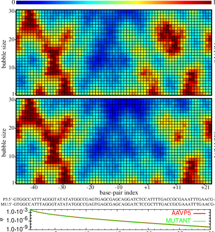
Figure 1: (color). The probability of bubble opening as function of bubble size and position for the AAVP5 promoter and the mutant sequence at 300 K. Probabilities in each row are normalized by a different factor $\phi(m)=\textrm{MAX}[\left\langle\theta_{i}^{[m]}\right\rangle_{\mu}]\textrm{ for }i\in[1,N]$ given in the lower panel. The 69 bp sequences start at index -46 and end at +23. The TSS is at +1, the mutation is at $(+1,+2)$ were (A,T) bases are replaced by (G,C). Contrary to ChoiNuc2004 , the mutation effect is very local.

The calculation of $z_{X}^{(i)}(y_{i})$ for a discrete set of $n_{\rm grid}$ values $y_{i}$ requires only $n_{\rm grid}^{2}$ function evaluations whenever $z_{X}^{(i-1)}$ is known. Hence, a total of $N\cdot n_{\rm grid}^{2}$ function evaluations are required instead of $n_{\rm grid}^{N}$ which is a huge improvement. Further increase can be obtained by introducing proper cut-offs for the numerical integration. We use integration boundaries such that for all $i$: $L<y_{i}<R$ and $|y_{i}-y_{i-1}|<d$, which we control by a single input parameter $\epsilon$: $d=\sqrt{\frac{2|\ln\epsilon|}{\beta K}}$, $L=-\frac{1}{a_{A}T}\ln\Big{[}\ \sqrt{\frac{|\ln\epsilon|}{\beta D_{AT}}}+1\Big{]}$, and $R=y_{0}+\sqrt{N}d$. Any configuration outside this range but with at least one base-pair closed will have a probability density smaller than $\epsilon/(Z-Z_{\Pi})$. A strong decrease in the parameter $\epsilon$ will only marginally increase the integration boundaries. We took $\epsilon=10^{-40}$ that is much smaller than necessary for our accuracy. After storing the following function values in matrices $M_{ij}^{(AT/GC)}\equiv\exp(-\beta[V_{\rm AT/GC}(L+i\Delta y)+W(L+i\Delta y,L+(i+j)\Delta y)])$ with $0\leq i\leq\textrm{INT}[(R-L)/\Delta y]$ and $-\textrm{INT}[d/\Delta y]\leq j\leq\textrm{INT}[d/\Delta y]$ we can reduce the integral operations for Eq. (6) (using Simpson’s rule) into inexpensive multiplication and addition operations only.

As a first investigation, we applied this new method on the adeno-associated viral P5 promoter and the mutant from Refs. ChoiNuc2004 using $y_{0}=1.5$ as opening threshold which corresponds to 2.1 Å  in real units. To make the comparison with MD which uses periodic boundary conditions (PBC), we replicated the chain at both ends, but only computed the statistics for the middle chain. This approach, is cheaper than true PBC which scales as $N\cdot(n_{\rm grid})^{3}$. The full probability matrix $\left\langle\theta_{i}^{[m]}\right\rangle_{\mu}$ was calculated for the middle sequence up to bubbles of size $m=50$. A fraction of this matrix is presented in Fig. 1 in a color plot. In agreement with Ref. ChoiNuc2004 we find preferential opening probabilities at the TSS site at +1 that vanishes after the mutation. But contrary to the results of Ref. ChoiNuc2004 , we find that the TSS is not at all the most dominant opening site. Stronger opening sensitivity is found at the -30 region. Moreover at variance with the previous established findings, Fig. 1 shows that the mutation effect is very local.

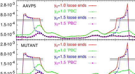
Figure 2: (color). The probabilities for bubbles larger than 10 bp for the AAVP5 promoter and the mutant at 300 K. Both semi-PBC (three-fold replicated system) and loose ends (single chain) are compared and two values for the opening threshold $y_{0}=1.0$ and $y_{0}=1.5$. MD results (black) for $y_{0}=1.5$ with PBC are also given with corresponding error-bars. A change of scale in the $y$ axis is applied to include the higher openings at the free boundaries. All results agree but are different from the less accurate results of ChoiNuc2004 . The mutation and the free boundaries only have a local impact on the bubble statistics.

In Fig. 2 we make a projection by looking at the probability $P_{i}\equiv\sum_{m=10}^{N-1}\left\langle\theta_{i}^{[m]}\right\rangle_{\mu}$ that at site $i$ one can find a bubble of size 10 or larger. We compared different boundary conditions and two values for $y_{0}$. In addition, we made the comparison with MD  by performing 100 simulations of 100 ns with different friction constants $\gamma$ in the Langevin MD and 10 simulations of 1 $\mu$s using Nosé-Hoover. The curves matched within the statistical errors and agreed with the integration method (see for instance Fig. 2 where the Langevin $\gamma=10$ results are plotted together with the results of the integration method).

We obtained relative errors around 10 % for Nosé-Hoover and Langevin with $\gamma=10$ and $5$ ps^-1. The errors of the $\gamma=0.05$ ps^-1, used in Ref. ChoiNuc2004 , were considerably larger due a stronger correlation between successive timesteps. The results of ChoiNuc2004 were based on 100 times fewer statistics. Hence, the corresponding errors in ChoiNuc2004 must have been 10 times larger which can explain the variance with our results. Another explanation could be that the results of ChoiNuc2004 are due to some out-of-equilibrium or dynamical effects. Such effects depend strongly on the choice of initial conditions, which poses the problem of defining biologically significant initial conditions and determining, in a meaningful way, the relevant time scale along which the simulations have to be carried to detect such non-equilibrium phenomena.

The principal error in the new method is mainly due to the finite integration steps. To estimate the accuracy, we compared $\Delta y=0.1$ and $0.05$ with the almost exact results of $\Delta y=0.025$. Using the TSS peak of the AAVP5 sequence with free boundaries as reference, we found that the systematic error drops from $\sim 5$ % to 0.03 % for CPU times of 40 minutes and 3 hours only. For comparison, the last accuracy would take about 200 years with MD on the same machine. The evaluation of larger bubbles becomes increasingly more difficult for MD. Bubbles of size 20 showed statistical errors $>100$ % while these were only slightly increased for the integration method. It is interesting to note that the 10 bp size is more or less the upper limit for which one get sufficient accuracy using MD, while it is a lower limit were its relation to biophysics becomes interesting Murakamiscience stressing the importance of our method.

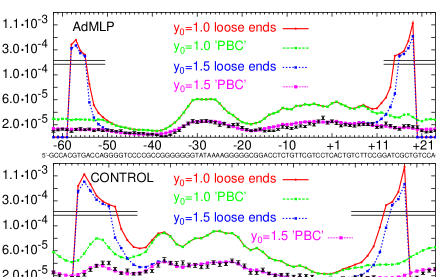
Figure 3: (color). Same as Fig. 2 for the 86 bp AdMLP and the 63 bp non-promoter control sequences. The biological non-active control sequence shows considerable opening probability, even more than the biological active AdMLP promoter.

Finally, we calculated the $P_{i}$ probabilities for the adenovirus major late promoter (AdMLP) and a control non promoter sequence (Fig. 3). Also here, our results violate the TSS conjecture. The TSS shows some opening, but cannot be assigned on basis of bubble profile only. Surprisingly, even the control sequence shows significant opening probabilities.

To conclude, we have shown that MD (or MC) encounters difficulties to give a precise indication of preferential opening sites. In particular, information of large bubbles is not easily accessible using standard methods. The method presented here is orders of magnitude faster than MD without imposing additional approximations. Using this method, we showed that the TSS is generally not the most dominant opening site for bubble formation. These results contradict foregoing conjectures based on less accurate simulation techniques. However, to address the title’s question, definitely, there are still many issues to be solved. Still, there is some chance that bubble dynamics rather than bubble statics is indicatory for the TSS. Speculatively, the previously found correlation could be justified using this argument. However, a statistical significant foundation for this is lacking and it is highly questionable whether the PBD model and this type of Langevin dynamics can give a sufficiently accurate description for the dynamics of DNA. The PBD model could and, probably, should be improved to give a correct representation of the subtile sequence specific properties of DNA. Base specific stacking interaction seems to give better agreement with some direct experimental observations Santiago . Also, the development of new experimental techniques is highly desirable. Our method is not limited to the PBD model or to bubble statistics only, but it works whenever the proper factorization (6) can be applied. Therefore, we believe that the technique presented here will remain of importance for the future investigations of bubbles in DNA and their biological consequences.

We thank Dimitar Angelov and David Dubbeldam for fruitful discussions. TSvE is supported by a Marie Curie Intra-European Fellowships (MEIF-CT-2003-501976) within the 6th European Community Framework Programme. SCL is supported by the Spanish Ministry of Science and Education (FPU-AP2002-3492), project BFM 2002-00113 DGES and DGA (Spain).

References

- (1) U. Dornberger, M. Leijon, and H. Fritzsche, J. Biol. Chem. 274, 6957 (1999).
- (2) C. J. Benham, Proc. Natl. Acad. Sci. USA 90, 2999 (1993); C. J. Benham, J. Mol. Biol. 255, 425 (1996).
- (3) C. H. Choi et al., Nucl. Acid Res. 32, 1584 (2004); G. Kalosakas et al., Eur. Phys. Lett. 68, 127 (2004).
- (4) M. Peyrard and A. R. Bishop, Phys. Rev. Lett. 62, 2755 (1989).
- (5) T. Dauxois, M. Peyrard, and A. R. Bishop, Phys. Rev. E 47, 684 (1993).
- (6) A. Campa and A. Giansanti, Phys. Rev. E 58, 3585 (1998).
- (7) K. S. Murakami et al., Science, 296, 1285 (2002).
- (8) S. Cuesta-Lopez et al, to be published