Oscillations in molecular motor assemblies

Abstract

Autonomous oscillations in biological systems may have a biochemical origin or result from an interplay between force-generating and visco-elastic elements. In molecular motor assemblies the force-generating elements are molecular engines and the visco-elastic elements are stiff cytoskeletal polymers. The physical mechanism leading to oscillations depends on the particular architecture of the assembly. Existing models can be grouped into two distinct categories: systems with a delayed force activation and anomalous force-velocity relations. We discuss these systems within phase plane analysis known from the theory of dynamic systems and by adopting methods from control theory, the Nyquist stability criterion.

1 Introduction

Oscillations are ubiquitous in biological systems. Examples range from circadian rhythms associated with external periodicities to autonomous bio-chemical [31] and mechano-chemical oscillators. Voltage oscillations in systems of ion channels embedded in a cell membrane are one of the most prominent examples for a biochemical oscillator. At the heart of its explanation within the Hodgkin-Huxley model [19] there is a negative differential current-voltage relation for the ion channels. Such biochemical oscillators are by now well studied [31]. Recently, there has been growing interest in mechano-chemical systems composed of visco-elastic biopolymer arrays and active molecular machines driven by the chemical cycle of ATP hydrolysis; these will be the focus of our contribution. We ask how the interplay between force-generation and energy-input by the molecular motors and the restoring forces and damping mechanisms provided by the biopolymer system may lead to oscillatory behavior.

There are many examples of functional units in cellular systems whose main components are molecular machines and visco-elastic elements. The part list of auditory hair bundles contains stereocilia (elastic rods composed of bundles of stiff biopolymers F-actin), myosin (a force-generating molecular motor) and mechanosensitive ion-channels. Spontaneous oscillations in such systems are by now well documented experimentally [27] and explained within simple theoretical models [10, 42]. This oscillatory behavior of hair bundles provides a mechanism for active amplification of acoustic signals [7]. Another example are eucaryotic cilia and flagella which are used by many small organisms to swim. Here the main structural element are axonemes, which consist of a cylindrical arrangement of elastically linked microtubules (another example for a stiff biopolymer) and an assembly of dynein motors located between neighboring microtubules. Forces generated by the dynein motors induce relative sliding between microtubules which in turn results into bending of the axonemes [5]. Oscillatory behavior in such systems is generic and intimately connected with a Hopf bifurcation [8]. Sarcomeres, the contractile units of muscle, are composed of two sets of protein filaments: myosin filaments (containing myosin motors) and actin filaments. The shortening of the sarcomere is achieved by the actin and myosin filaments sliding over one another. While the primary function of most types of muscle is to generate a unidirectional force, some muscle (notably the asynchronous, also known as fibrillar or myogenic insect flight muscle) are specialized on autonomous oscillatory contraction. The oscillation mechanism usually includes a number of regulatory proteins that constitute the delayed stretch-activation mechanism. However, oscillations were also observed in skeletal muscle fibrils, mostly under non-physiological conditions [32]. Theoretical studies show that even skeletal muscle myosin could produce oscillatory motion [14, 13, 40], which is normally not observable because the contributions of different sarcomeres cancel out. However, a sudden change in applied load can lead to synchronization of sarcomeres and the oscillations become observable for a certain period of time [15]. Assemblies of molecular motors and stiff biopolymers also play an essential role during cell division. The duplicated genome is segregated into two daughter cells through the action of the mitotic spindle. It consists of fibres (microtubule bundles) radiating from two poles and meeting at the equator in the middle. The spindle poles have been found to oscillate [16]. Recently it has been shown that these oscillations are again due to an interplay between force-generating and elastic elements [17].

Here we will focus on a discussion of the generic features of oscillations in molecular motor assemblies to highlight the common physical mechanisms. For more system specific and detailed discussions we refer the reader to the literature. The defining elements of molecular motor assemblies are: (i) an external energy source driving the system towards a non-equilibrium steady state, (ii) viscoelastic elements providing restoring forces and damping mechanisms, (iii) possibly force-dependent biochemical reactions which allow for switching between different states of the molecular motor assembly. The particular interconnection between these components gives rise to the system response which may be controlled by the biochemical reaction rates. Defined as such there are obvious analogies to system and control theory which is a well established discipline in engineering [12]. In particular, linear system analysis is a most fruitful concepts which we will also employ to characterize the system’s dynamic response.

The mechanisms for oscillations in chemochemical models discussed in the literature can be grouped into two distinct categories. In delayed force activation systems an imposed displacement $x$ is transduced into a force $f$ with some delay time $\tau$ (Debye relaxator). As such the system would evolve towards a time-independent steady state. Oscillatory response is achieved only after coupling the Debye relaxator to other dynamic elements with either a negative stiffness or some inertial (massive) load. Anomalous force-velocity relations are an alternative route towards oscillatory behavior. This means that an assembly of motors can move with two different velocities (e.g., one positive and one negative) under the same load [35]. If attached to an external spring, the motors will move forwards until the spring force exceeds a certain threshold, then they will switch to the other stable state and slide backwards, until another threshold is reached and so the cycle repeats [24].

2 Response Functions

To assess the stability of an active mechanical system like an insect muscle attached to the wing or the dynein motor acting between two tubulin filaments in a flagellum, the response function can be defined the following way. We connect the active system to a mechanical actuator that keeps its length at the desired point of operation and at the same time imposes small oscillations with the amplitude $x_{0}$ around that point

$$\Delta x(t)={\rm Re\,}x_{0}e^{i\omega t}\;.$$ (1)

Fur sufficiently small oscillations the system responds with a force that oscillates with the same frequency

$$\left<\Delta f(t)\right>={\rm Re\,}f_{0}e^{i\omega t}\;.$$ (2)

Here $\left<\right>$ denote an ensemble average over different realizations of the response of the stochastic system. Note that the sign in the exponent of the Fourier transform was chosen in the way that is most common in the literature on muscle, although it is opposite to the convention frequently used in physics. We define the force in the way that it is positive if the motor system is being pulled upon in the direction of positive $x$. In the limit of small amplitude $x_{0}$, the relation becomes linear

$$f_{0}=G(\omega)x_{0}\;,$$ (3)

with the frequency dependent response function or modulus $G(\omega)$. Here the real part of $G$ corresponds to the elastic and the imaginary part to the dissipative response. For a spring with a spring constant $k$ the response function is $G(\omega)=k$ and for a damping element (“dashpot”) $G(\omega)=i\omega\gamma$.

One may also encounter a situation where for a given force $f$ one is observing the displacement $x$ for various realizations of the system response,

$$\left<x(\omega)\right>=\chi(\omega)\,f(\omega)\;.$$ (4)

The two response functions become equivalent

$$\chi(\omega)=1/G(\omega)$$ (5)

if the following two conditions are fulfilled. First, the system needs to be stable, so that the operational point is the same regardless whether the position or the force is imposed. Second, the systems are large enough such that variance of the stochastic variable is small compared to its mean.

3 The Nyquist stability criterion

The Nyquist stability criterion is a convenient tool to analyze the stability of a dynamical system if the complex response function $G(\omega)$ is known over the whole frequency range. It states that the system is dynamically unstable if the plot of ${\rm Im\,}G(\omega)$ vs. ${\rm Re\,}G(\omega)$ (Nyquist plot, sometimes also called Cole-Cole plot) encircles the coordinate origin in clockwise direction. It is frequently used in engineering, especially for the stability analysis of closed feedback loops in electrical circuits [12].

To derive it we first note that the system is dynamically unstable if it starts oscillating with a growing amplitude in the absence of a force, $\left<f\right>=0$. This is the case if there exists an eigenmode, i.e., a complex solution of the equation $\left<f(x_{0},\omega)\right>=0$ with ${\rm Im\,}\omega<0$, since then the corresponding solution $\Delta x(t)\propto e^{i\omega t}$ obviously diverges for $t\to+\infty$. This means that $G(\omega)$ has a zero and $\chi(\omega)$ has a pole in the lower half-plane with ${\rm Im\,}\omega<0$. The Nyquist criterion is based on the fact that $G(\omega)$ is an analytical complex function and utilizes Cauchy’s theorem to relate the number of zeros in the negative imaginary $\omega$ half-plane to the contour of $G(\omega)$, evaluated for real values of $\omega$.

According to Cauchy’s theorem, the change of phase along a closed contour in clockwise direction in the complex $\omega$ plane equals

$$\oint d(\arg G(\omega))=2\pi\left(-\sum_{k=1}^{N_{z}}n_{z,k}+\sum_{k=1}^{N_{p}}n_{p,k}\right)\;,$$ (6)

where $N_{z}$ is the number of encircled zeros of $G(\omega)$, $N_{p}$ the number of poles and $n_{z,k}$ and $n_{p,k}$ their multiplicities. For example, the function $G(\omega)=i\omega\gamma$ has a single zero ($N_{z}=1$) with multiplicity 1 ($n_{z,1}=1$) at $\omega=0$. Accordingly, it changes its phase by $-2\pi$ on a clockwise circle around the origin. The function $G(\omega)=-m\omega^{2}$, on the other hand, has a zero with multiplicity $n_{z,1}=2$ at $\omega=0$ and it changes its phase by $-4\pi$ on the same circle.

We apply Cauchy’s theorem to a path that runs along the real $\omega$ axis from $\omega=-\infty$ to $\omega=+\infty$ and close it in the negative imaginary plane as shown in Fig. 1a. We further note that in a real system $G(\omega)$ can have no poles in the negative imaginary half-plane, because they would imply an infinite force response to a finite displacement growing in time. Therefore, any phase change along that path indicates a zero with ${\rm Im\,}\omega<0$, and therefore a dynamical instability.

Figure 1: a) The integration path for Eq. 6 in the complex $\omega$ plane. Encircled zeros (marked ”$\times$”) correspond to unstable eigenmodes. b) $G$ in the complex plane, with $\omega$ as a parameter. The points denoted as A,B and C correspond to a negative, 0 and a positive value of $\omega$. The curve shown has a typical shape measured on insect flight muscle [26].

Now we can look at the same path in the complex $G$ plane, i.e., ${\rm Im\,}G(\omega)$ plotted against ${\rm Re\,}G(\omega)$, where $\omega$ acts as a curve parameter. The strand along the real axis in the $\omega$ plane corresponds to the $({\rm Re\,}G(\omega),{\rm Im\,}G(\omega))$ curve, with $\omega$ taking real values values from $-\infty$ to $\infty$. In case $G(-\infty)\neq G(\infty)$, we close the path in the positive real half-plane (Fig. 1b), which corresponds to the closure in the ${\rm Im\,}\omega<0$ half-plane. A change of phase of $G$ along the path in the $\omega$ plane by a multiple of $-2\pi$ directly represents the same number of origin encirclements in the $G$ plane. Therefore, it follows from (6) that the complex $G(\omega)$ curve encircles the coordinate origin $\sum_{1}^{N_{z}}n_{z,k}$ times in clockwise direction.

Note that the curve is symmetric with respect to the real axis. This becomes evident from the following consideration. Because $G(t)$ is a real function, its Fourier transformed has to fulfill the following symmetry relation:

$$G(-\omega^{*})=G^{*}(\omega)\;.$$ (7)

For real $\omega$ values, this means $G^{*}(\omega)=G(-\omega)$, and for each $G$ value its complex conjugate is part of the curve as well.

An additional consequence of the Nyquist criterion is that the origin can only be encircled in clockwise direction, because $G$ contains zeros but no poles in the relevant region.

4 Delayed force activation

One type of models, often used to explain oscillations generated by molecular motors involves a delayed force activation mechanism. This means that when the system is displaced by the distance $x$ in one direction, it develops a restoring force $f$, however not instantaneously, but according to a differential equation like:

$$\frac{df}{dt}=(K_{A}x-f)/\tau\;.$$ (8)

Here $\tau$ represents the time constant with which the force reacts to a position change and $K_{A}$ an effective steady state stiffness of the active system. There are many different physical mechanisms that can produce a delayed force response (Fig. 2):

1. Stretch-activation of insect flight muscle: a number of regulatory proteins facilitate the activation of myosin motors following a mechanical stretch (a relative displacement of thin filaments relative to thick) [33, 11, 1]. After the activation, the development of force does not follow instantaneously, but with a certain time constant, typically with the attachment rate of motors.

2. In a sarcomere a position change can bring myosin heads closer to the accessible actin sites [39, 38]. This mechanism has been proposed for insect flight muscle [44], although experiments have later refuted it in many cases [36].

3. The switching of bound myosin heads between two conformations with different detachment rates can lead to an effective stretch-dependent activation [40, 9].

4. The opening of a mechanically gated ion channel can cause the influx of calcium ions, which then promote channel reclosure. This is called the fast adaptation mechanism in auditory hair cells and can generate spontaneous hair bundle oscillations [34, 20, 10, 42]. If the hair cell is on the verge of spontaneous oscillations (i.e., close to a Hopf bifurcation) it has the best sensitivity, dynamic range and frequency selectivity [7].

5. Calcium ions, entering the ion channel, can reduce the force generated by adaptation motors of type myosin 1C [3], a mechanism known as slow adaptation in auditory hair cells [21, 29, 28].

6. Some models for flagellar dynein are based on a strain-controlled [25] or curvature-controlled [5] activation.

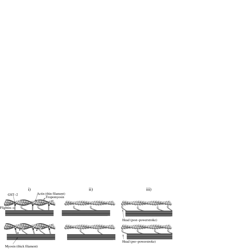
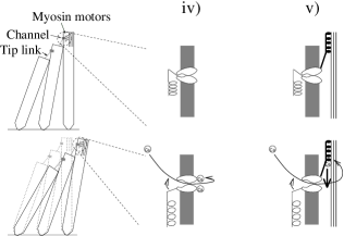
Figure 2: Different biological mechanism that lead to delayed force activation: i) Stretch activation in insect flight muscle, after [30]. The applied stretch activates myosin mechanically through conformational changes involving flightin, GST-2, troponin-H and tropomyosin. ii) The alternative match-mismatch mechanism, where the myosin heads are activated when they are brought to appropriate positions along the actin helix. iii) The mechanism involving switching of myosin heads between two bound conformations. A stretch brings more myosin heads into the pre-powerstroke state, which is less likely to detach from actin, and therefore the total number of active heads increases [40]. iv) The fast adaptation mechanism in auditory hair cells. When the transduction channel opens, calcium ions enter and promote the reclosure of the channel. v) The slow adaptation mechanism in auditory hair cells: calcium ions entering the cells reduce the force generated by myosin motors, therefore they slip back and the channel is more likely to close again.

The solution of (8) can be expressed with a Green’s function $G_{A}(t)$, so that

$$f(t)=\int_{-\infty}^{t}G_{A}(t-t^{\prime})x(t^{\prime})dt^{\prime}\qquad\mbox{with}\qquad G_{A}(t)=\frac{K_{A}}{\tau}e^{-t/\tau}\;.$$ (9)

Such behavior is well known from many branches in physics under the term Debye relaxator. The corresponding response function

$$G_{A}(\omega)=\frac{K_{A}}{1+i\omega\tau}$$ (10)

is represented by a circle in a Nyquist plot (see Fig. 3 (a)).

Figure 3: Nyquist plots (also called Cole-Cole plots or vector modulus plots) of the response function of a system with delayed force activation. a) The response function of the delayed force activation alone, given by Eq. (10). b) Response function of the delayed force activation, combined with a damping element, $G_{A}+G_{D}$ (spring $K=5K_{A}$, dashpot with a constant $\gamma/K=100/\tau$). c) System as in (b), additionally combined with an element with negative effective elasticity; $G_{A}+G_{D}+G_{N}$ ($K_{1}=-0.2K_{A}$). d) Response function $G_{A}+G_{I}$ of the system with delayed force activation, combined with a damped inertial oscillator ($\omega_{0}=10/\tau$, $K=2K_{A}$, $\beta=10/\tau$).

It does have a negative imaginary part, however, the real part is always positive. Hence the Nyquist plot of $G_{A}(\omega)$ cannot encircle the coordinate origin and thereby satisfy the Nyquist criterion for an instability. The stationary state of the Debye relaxator simply is a time-independent displacement $x^{\star}=f/K_{A}$. Note, that a dynamics with a one-dimensional phase space, i.e. first order differential equations of the form $df/dt=x(f)$, is either monotonic or constant [37]. Only if the dynamic variable is on a circle or if the phase space has more than two dimensions oscillations emerge as possible solutions.

One way to make the system unstable is to connect the active mechanism with an element that shifts the Nyquist plot towards negative values on the real axis; for an illustration of the type of connection see Fig. 3. This can be trivially achieved through an element with a negative effective stiffness, or, as we will show below, through an inertial load.

Figure 3 shows the response function of the delayed activation system (10), combined with different elements. The first is an element consisting of a spring (constant $K$) and a dashpot (damping coefficient $\gamma$) in series. Their combined response function reads

$$G_{D}(\omega)=\left(\frac{1}{K}+\frac{1}{i\omega\gamma}\right)^{-1}\;.$$ (11)

A second element we connect to the motor assembly is an element with negative effective elasticity,

$$G_{N}(\omega)=K_{1}<0\;.$$ (12)

The third element is a damped inertial oscillator (a spring connected to a mass, with an additional damping element connecting both to a fixed point). The response function of such an element reads

$$G_{I}(\omega)=\left(\frac{1}{K}+\frac{1}{-m\omega^{2}+i\omega\gamma}\right)^{-1}=K\left(1-\frac{\omega_{0}^{2}}{\omega_{0}^{2}-\omega^{2}+i\beta\omega}\right)$$ (13)

with $\omega_{0}^{2}=K/m$ and $\beta=\gamma/m$.

Negative stiffness can be generated by the gating compliance of ion channels [22, 29] or by motors switching between two states [18, 40]. Inertial load is the likely mechanism of ensuring an instability in insect flight muscle [41]. Also in many types of hair cells, no negative stiffness has been observed, but as the hair bundle is often attached to the tectorial membrane, inertial load could play an important role as well [2].

5 Anomalous force-velocity relations

A class of models that were frequently discussed in relation to dynamical instabilities in systems of molecular motors is based on an anomalous force-velocity relation, meaning that a group of coupled motors produces a force that displays a region with negative slope as a function of velocity. Models for dynein [6], myosin [43], propulsion by actin polymerization [4], mitotic spindle oscillations [17] as well as generic motors [23, 24] were based on this mechanism.

A common feature of such models is translational invariance, meaning that the force $f(t)$ does not depend on the position $x$, but only on the velocity $v$ and the history thereof. The translational invariance can be achieved even on periodic tracks (like actin filaments) if the motors (myosin heads) are arranged incommensurate to the track periodicity [23].

An instructive example of a system displaying an anomalous force-velocity relation is a two-state cross-bridge model for motors like myosin. In this model, motors can attach to actin in a forward-leaning position with rate $r_{\rm a}$, then quickly undergo a conformational change, which makes them strained. When the filaments moves, this strain changes with time (for forward-running motors, it decreases), and when the motor eventually detaches with a strain-dependent rate $r_{\rm d}(\xi)$ the cycle can repeat. Each motor generates a force $k\xi$, proportional to its strain $\xi$. A full description of this system requires Master equations for the probability of a motor for being in the detached state ($\Phi_{\rm d}$) and for the probability density of a motor for being in the attached state with strain $\xi$ ($\Phi_{\rm a}(\xi)$).

$$\left(\partial_{t}-v\partial_{\xi}\right)\Phi_{\rm a}(\xi,t) = \Phi_{\rm d}(t)r_{\rm a}P(\xi)-\Phi_{\rm a}(\xi,t)r_{\rm d}(\xi)$$ (14a)

$$\partial_{t}\Phi_{\rm d}(t) = -\Phi_{\rm d}(t)r_{\rm a}+\int_{-\infty}^{\infty}d\xi\,\Phi_{\rm a}(\xi,t)r_{\rm d}(\xi)\,,$$ (14b)

Both probabilities are not independent but normalized such that $\Phi_{\rm d}+\int_{-\infty}^{\infty}\Phi_{\rm a}(\xi)d\xi=N$ gives the total number of motors. $P(\xi)$, normalized as $\int_{-\infty}^{\infty}P(\xi)d\xi=1$ is the distribution of strains on newly attached motors, with an expectation value $d=\int_{-\infty}^{\infty}P(\xi)\xi d\xi$. A general analytical solution for the stationary state of these equations is given in [43].

To illustrate the key physical features of this model we neglect the strain-dependence of the attachment probability and assume that all attached motors have the same strain $y(t)$,

$$\Phi_{\rm d}(\xi,t)=n(t)\,\delta(\xi-y(t))\;.$$ (14o)

Then the number of attached motors $n(t)$ is related to the number of detached motors by $\Phi_{\rm d}(t)=N-n(t)$. Upon inserting these relations into Eqs.14a,b , multiplying Eq.14a with $\xi$ and integrating over all values of $\xi$ one obtains a simplified set of dynamic equations for $y(t)$ and $n(t)$:

$$\dot{y} = [d-y]\frac{N-n}{n}r_{\rm a}-v$$ (14pa)

$$\dot{n} = [N-n]r_{\rm a}-nr_{\rm d}(y)$$ (14pb)

The external force on the system, which equals the total force produced by the motors, is given as

$$f=-nky$$ (14pq)

where $k$ denotes the spring constant of each motor. These are nonlinear flow equations with a two-dimensional phase space consisting of the strain $y(t)$ and the number density $n(t)$ of the attached motors. For a constant velocity $v$, they always have a stable stationary solution. However, if we take the system consisting of the group of motors, coupled to an external spring with a spring constant $K$, so that the force equilibrium states $f+Kx=0$, we obtain a new system of two nonlinear equations for two independent variables (e.g., $x$ and $n$). Depending on the parameter values, they can have a stable fixed point or a limit cycle (oscillatory steady state). These two examples are shown in Fig. 4.

Figure 4: Numerical solution of the equations of motion (14pa,b) for the system of motors, coupled to a spring with a constant $K=0.4\times Nk$ (a) and $K=0.3\times Nk$ (b). The force-dependent detachment rate was chosen as $r_{d}(y)=r_{a}\exp(2(x/d)^{2}-2)$. The system has a stable fixed point in the first case and an unstable one, surrounded by a limit cycle, in the second case.

In the following we will again use the stability analysis of linear response functions to characterize the system. In the absence of an external velocity ($v=0$), Eqs. 14pa,b have a stable stationary solution with $y_{0}=d$ and $n_{0}=\frac{r_{\rm a}}{r_{\rm a}+r_{\rm d}(d)}N$. For small values of $v$ we can linearize the flow equations to

$$\dot{y} = -r_{\rm d}(d)\Delta y-v$$ (14pra)

$$\dot{n} = -n_{0}r_{\rm d}^{\prime}(d)\Delta y-(r_{\rm a}+r_{\rm d}(d))\Delta n$$ (14prb)

where $\Delta y=y-y_{0}$ and $\Delta n=n-n_{0}$. These equations have two negative eigenvalues, $-\lambda_{1}=-r_{\rm d}(d)$ and $-\lambda_{2}=-r_{\rm a}-r_{\rm d}(d)$. The solution of the coupled system then has the form

$$\Delta y(t) = -\int_{-\infty}^{t}dt^{\prime}e^{-\lambda_{1}(t-t^{\prime})}v(t^{\prime})$$ (14prsa)

$$\Delta n(t) = \frac{n_{0}r_{\rm d}^{\prime}(d)}{r_{\rm a}}\,\int_{-\infty}^{t}dt^{\prime}\left[e^{-\lambda_{1}(t-t^{\prime})}v(t^{\prime})-e^{-\lambda_{2}(t-t^{\prime})}\right]v(t^{\prime})$$ (14prsb)

The force can be determined as

$$f(t)=-nky=f_{0}+\int_{-\infty}^{t}dt^{\prime}kn_{0}\left[(1-\alpha)e^{-\lambda_{1}(t-t^{\prime})}+\alpha e^{-\lambda_{2}(t-t^{\prime})}\right]v(t^{\prime})\;.$$ (14prst)

Where $\alpha=\frac{dr_{\rm d}^{\prime}(d)}{r_{\rm a}}$ is a dimensionless coefficient. With a more precise solution, or with more complex model equations, the solution could contain more than two relaxation constants, but its basic form would remain. Inserting a stationary velocity ($v(t)\equiv\mbox{const}$) in Eq. (14prst) one can see that the system displays an anomalous stationary force velocity relation if $\alpha$ is sufficiently large that

$$\frac{1-\alpha}{\lambda_{1}}+\frac{\alpha}{\lambda_{2}}<0$$ (14prsu)

The response function in Fourier space follows from Eq. (14prst):

$$G(\omega)=n_{0}k(1-\alpha)\frac{i\omega}{\lambda_{1}+i\omega}+n_{0}k\alpha\frac{i\omega}{\lambda_{2}+i\omega}$$ (14prsv)

In the limit $\omega\to\infty$, the response is always that of the elastic elements involved, $G=n_{0}k$. Figure 5 shows the resulting Nyquist plot for two scenarios: with a normal and an anomalous force-velocity relation. In case of an anomalous force velocity relation the curve encircles the origin and the system is dynamically unstable.

Figure 5: Nyquist plots (Cole-Cole plots, vector modulus plots) of the response function $G(\omega)$ (14prsv) for $\alpha=0$ (a) and $\alpha=5$ (b). Other parameter values: $r_{\rm d}(d)=r_{\rm a}$, implying $\lambda_{2}=2\lambda_{1}$. Negative $\omega$ values are shown with dashed lines. The system in (a) is dynamically stable, because the curve does not encircle the origin, while that in (b) oscillates spontaneously.

If the assembly of motors is coupled to an elastic element (spring constant $K$), the curve in the Nyquist plot is shifted to the right by the amount $K$. There is a critical value of $K$ at which the oscillations stop. In the example shown in Fig. 4, this value would lie between those used in both diagrams. At the transition point the system exhibits a Hopf bifurcation [24, 17].

In summary, based on the foregoing discussion, we feel that a combination of methods from the engineering sciences like control theory and methods from the theory of dynamic systems may be fruitful for future analysis of molecular motor assemblies or other functional units in cellular systems.

Acknowledgment

We have benefitted from discussions with Tom Duke, Frank Jülicher, Thomas Franosch and Franz Schwabl. This work was supported by the Slovenian Office of Science (Grants No. Z1-4509-0106-02 and P0-0524-0106).

References

References

- [1] B. Agianian, U. Kržič, F. Qiu, W. A. Linke, K. Leonard, and B. Bullard. A troponin switch that regulates muscle contraction by stretch instead of calcium. EMBO J., 23:772–779, 2004.
- [2] S. Authier and G. A. Manley. A model of frequency tuning in the basilar papilla of the Tokay gecko, Gekko gecko. Hear. Res., 82:1–13, 1995.
- [3] C. Batters, M. I. Wallace, L. M. Coluccio, and J. E. Molloy. A model of stereocilia adaptation based on single molecule mechanical studies of myosin I. Philos. Trans. R. Soc. Lond. B Biol. Sci., 359:1895–1905, 2004.
- [4] A. Bernheim-Groswasser, J. Prost, and C. Sykes. Mechanism of actin-based motility: a dynamic state diagram. Biophys. J., 89:1411–1419, 2005.
- [5] C. J. Brokaw. Bend propagation by a sliding filament model for flagella. J. Exp. Biol., 55:289–304, 1971.
- [6] C. J. Brokaw. Molecular mechanism for oscillation in flagella and muscle. Proc. Natl. Acad. Sci. USA, 72:3102–3106, 1975.
- [7] S. Camalet, T. Duke, F. Jülicher, and J. Prost. Auditory sensitivity provided by self-tuned critical oscillations of hair cells. Proc. Natl. Acad. Sci. USA, 97:3183–3188, 2000.
- [8] S. Camalet, F. Jülicher, and J. Prost. Self-organized beating and swimming of internally driven filaments. Phys. Rev. Lett., 82:1590, 1999.
- [9] K. B. Campbell, M. V. Razumova, R. D. Kirkpatrick, and B. K. Slinker. Nonlinear myofilament regulatory processes affect frequency-dependent muscle fiber stiffness. Biophys. J., 81:2278–2296, 2001.
- [10] Y. Choe, M. O. Magnasco, and A. J. Hudspeth. A model for amplification of hair-bundle motion by cyclical binding of Ca2+ to mechanoelectrical-transduction channels. Proc. Natl. Acad. Sci. USA, 95:15321–15326, 1998.
- [11] M. Dickinson, G. Farman, M. Frye, T. Bekyarova, D. Gore, D. Maughan, and T. Irving. Molecular dynamics of cyclically contracting insect flight muscle in vivo. Nature, 433:330–334, 2005.
- [12] R. C. Dorf. Modern Control Theory. Addison Wesley Publishing Company, 1967.
- [13] T. Duke. Cooperativity of myosin molecules through strain-dependent chemistry. Philos. Trans. R. Soc. Lond. B Biol. Sci., 355:529–538, 2000.
- [14] T. A. J. Duke. Molecular model of muscle contraction. Proc. Natl. Acad. Sci. USA, 96:2770–2775, 1999.
- [15] K. A. P. Edman and N. A. Curtin. Synchronous oscillations of length and stiffness during loaded shortening of frog muscle fibres. J. Physiol., 534:553–563, 2001.
- [16] S. W. Grill, P. Gonczy, E. H. Stelzer, and A. A. Hyman. Polarity controls forces governing asymmetric spindle positioning in the Caenorhabditis elegans embryo. Nature, 409:630–633, 2001.
- [17] S. W. Grill, K. Kruse, and F. Jülicher. Theory of mitotic spindle oscillations. Phys. Rev. Lett., 94:108104, 2005.
- [18] T. L. Hill. Theoretical formalism for the sliding filament model of contraction of striated muscle. Part I. Prog. Biophys. Mol. Biol., 28:267–340, 1974.
- [19] A. L. Hodgkin and A. F. Huxley. A quantitative description of membrane current and its application to conduction and excitation in nerve. J. Physiol., 117:500–544, 1952.
- [20] J. R. Holt and D. P. Corey. Two mechanisms for transducer adaptation in vertebrate hair cells. Proc. Natl. Acad. Sci. USA, 97:11730–11735, 2000.
- [21] J. Howard and A. J. Hudspeth. Mechanical relaxation of the hair bundle mediates adaptation in mechanoelectrical transduction by the bullfrog’s saccular hair cell. Proc. Natl. Acad. Sci. USA, 84:3064–3068, 1987.
- [22] J. Howard and A. J. Hudspeth. Compliance of the hair bundle associated with gating of mechanoelectrical transduction channels in the bullfrog’s saccular hair cell. Neuron, 1:189–199, 1988.
- [23] F. Jülicher and J. Prost. Cooperative molecular motors. Phys. Rev. Lett., 75(13):2618–2621, 1995.
- [24] F. Jülicher and J. Prost. Spontaneous oscillations of collective molecular motors. Phys. Rev. Lett., 78:4510, 1997.
- [25] K. E. Machin. Wave propagation along flagella. J. Exp. Biol., 35:796–806, 1958.
- [26] K. E. Machin and J. W. S. Pringle. The physiology of insect fibrillar muscle III. The effect of sinusoidal changes of length on a beetle flight muscle. Proc. R. Soc. Lond. B, 152:311–330, 1960.
- [27] P. Martin, D. Bozovic, Y. Choe, and A. J. Hudspeth. Spontaneous oscillation by hair bundles of the bullfrog’s sacculus. J. Neurosci., 23:4533–4548, 2003.
- [28] P. Martin, A. J. Hudspeth, and F. Jülicher. Comparison of a hair bundle’s spontaneous oscillations with its response to mechanical stimulation reveals the underlying active process. Proc. Natl. Acad. Sci. USA, 98:14380–14385, 2001.
- [29] P. Martin, A. D. Mehta, and A. J. Hudspeth. Negative hair-bundle stiffness betrays a mechanism for mechanical amplification by the hair cell. Proc. Natl. Acad. Sci. USA, 97:12026–12031, 2000.
- [30] D. W. Maughan and J. O. Vigoreaux. An integrated view of insect flight muscle: Genes, motor molecules, and motion. News Physiol. Sci., 14:87–92, 1999.
- [31] J. D. Murray. Mathematical Biology. Springer Verlag, Heidelberg, 3rd edition, 2002.
- [32] N. Okamura and S. Ishiwata. Spontaneous oscillatory contraction of sarcomeres in skeletal myofibrils. J. Muscle Res. Cell Motil., 9:111–119, 1988.
- [33] J. W. S. Pringle. The Croonian Lecture, 1977. Stretch activation of muscle: function and mechanism. Proc. R. Soc. Lond. B, 201:107–130, 1978.
- [34] A. J. Ricci, Y. C. Wu, and R. Fettiplace. The endogenous calcium buffer and the time course of transducer adaptation in auditory hair cells. J. Neurosci., 18:8261–8277, 1998.
- [35] D. Riveline, A. Ott, F. Julicher, D. A. Winkelmann, O. Cardosso, J. J. Lacapere, S. Magnusdottir, J.-L. Viovy, L. Gorre-Talini, and J. Prost. Acting on actin: the electric motility assay. Eur. Biophys. J., 27:403, 1998.
- [36] J. M. Squire. Muscle filament lattices and stretch-activation: the match-mismatch model reassessed. J. Muscle Res. Cell Motil., 13:183–189, 1992.
- [37] S. H. Strogatz. Nonlinear dynamics and Chaos: with applications to physics, biology, chemistry, and engineering. Addison-Wesley, Reading, Mass., 1994.
- [38] N. Thomas and R. A. Thornhill. Stretch activation and nonlinear elasticity of muscle cross-bridges. Biophys. J., 70:2807–2818, 1996.
- [39] N. Thomas and R. A. Thornhill. The physics of biological molecular motors. J. Phys. D., 31:253–256, 1998.
- [40] A. Vilfan and T. Duke. Instabilities in the transient response of muscle. Biophys. J., 85:818–826, 2003.
- [41] A. Vilfan and T. Duke. Synchronization of active mechanical oscillators by an inertial load. Phys. Rev. Lett., (91):114101, 2003.
- [42] A. Vilfan and T. Duke. Two adaptation processes in auditory hair cells together can provide an active amplifier. Biophys. J., 85:191–203, 2003.
- [43] A. Vilfan, E. Frey, and F. Schwabl. Force-velocity relations of a two-state crossbridge model for molecular motors. Europhys. Lett., 45:283–289, 1999.
- [44] J. S. Wray. Filament geometry and the activation of insect flight muscles. Nature, 280:325–326, 1979.