Ring Identification and Pattern Recognition in Ring Imaging Cherenkov (RICH) Detectors

Abstract

An algorithm for identifying rings in Ring Imaging Cherenkov (RICH) detectors is described. The algorithm is necessarily Bayesian and makes use of a Metropolis-Hastings Markov chain Monte Carlo sampler to locate the rings. In particular, the sampler employs a novel proposal function whose form is responsible for significant speed improvements over similar methods. The method is optimised for finding multiple overlapping rings in detectors which can be modelled well by the LHbC RICH toy model described herein.

1 Introduction

This article describes an algorithm for identifying rings among photons such as may be observed by Ring Imaging Cherenkov (RICH) detectors in high energy physics experiments. The performance of the algorithm is demonstrated in the context of the LHbC RICH simulation described in Section 10. (Not the LHCb experiment [1, 2]) There are many examples of applications for ring finding pattern recognition both within high energy particle physics [3, 4, 5, 6] and without [7, 8].

The first half of the article is entirely devoted to defining what all ring finders actually are. The second half of the article shows how the idealised ring finder of the first half can be realised by a real algorithm, the “ring-finder”, to within a good approximation.

We begin with some very simple but very important comments about pattern recognition in general, and then link these to the specific case of identifying rings in collections of dots.

The general comments about pattern recognition will make it clear that meaningful ring identification can only take place in the context of a well defined model for the process believed to have generated the data containing the ring images.

We therefore go on to describe a model of the way that charged particles passing through a radiator lead to rings of Cherenkov photons being detected on imaging planes. In describing this model, we are forced to make explicit our definitions of rings (both “reconstructed” and “real”) and of hits. We are also forced to write down the constituents of the probability distributions which relate them both. In terms of these distributions we are then able to write down the goal of an “ideal” ring finder in an unambiguous way. A devout Bayesian could justly say that there is little or nothing innovative in this first half of the article – it being composed largely of definitions and truisms.

The second half of the article sets out to achieve the goals of the first half, i.e. the creation an actual ring finding algorithm matching the idealised one as closely as possible.

The method chosen is a Metropolis-Hastings Monte Carlo (MHMC) sampling of a particular posterior distribution defined in the first half of the article. MHMC samplings in ring finders are not new [3] but their performance is strongly dependent on the choice of the so-called proposal distribution(s) they make use of (defined later). Indeed, the only freedom that one has in implementing the MHMC sampler, is in the definition of the proposal distribution(s) to be used – and so almost all of the second half of the article is devoted to describing the one used here.

Finally in Section 6 there are some examples of reconstructed rings.

A short note concerning common misconceptions about MHMC proposal distributions:

Among people who have not used MHMC samplers frequently, there is a common perception that proposal distributions appear to introduce a level of arbitrariness into the sampler or its results, and there are often questions or confusion about the manner in which they affect the results of the sampler. The short answer is that in the limit of large times (i.e. a large number of samples) the choice of proposal distributions has no effect at all on the results of the sampler! However, differences are seen after short times (small numbers of samples). A clever choice of proposal function allows you to get good results in a short time (seconds) whereas a bad choice might require hours, weeks or even years of CPU time before convergence of the fit for a single event. The motivation for choosing good MHMC proposal functions is thus a desire for efficiency in the sampler – not a desire to introduce some fancy abritrariness or personal prejudices into it.

2 Pattern Recognition and Ring Identification

The single most important thing to recognise when pattern matching is that:

It is impossible to recognise a pattern of any kind until you have an idea of what it is you are looking for.

To give a simple example from the context of ring finding: What rings should a ring finding pattern matcher identify in part (a) of figure 1?

Figure 1: What rings should we see in (a)? Are there two large concentric rings as indicated in (b)? Perhaps there are three small rings of equal radii as indicated in (c).

The answer must depend on what rings we expect to see!

Equivalently, the answer must depend on the process which is believed to have lead to the dots being generated in the first place. If we were to know without doubt that the process which generated the rings which generated the dots in (a) were only capable of generating large concentric rings, then only (b) is compatible with (a). If we were know without doubt that the process were only capable of making small rings, then (c) is the only valid interpretation. If we know the process could do either, then both (b) and (c) might be valid, though one might be more likely than the other depending on the relative probability of each being generated. Finally, if we were to know that the process only generated tiny rings , then there is yet another way of interpreting (a), namely that it represents 12 tiny rings of radius too small to see.

So any ring finding pattern matcher must incorporate knowledge of the process it assumes lead to the production of the dots in the first place.

Inevitably it is impossible to know every detail of the process leading to the generation of the dots, so in practice a ring finding pattern matcher must at the very minimum have a working model of the process that leads to the generation of the dots.

3 Rings of Cherenkov Photons in RICH Detectors.

When a charged particle traverses a medium at a speed greater than the speed of light in that medium, it emits Cherenkov photons at a constant angle to its line of flight (but at uniformly random azimuthal angles). With an appropriate optical set-up, it may be arranged that all the photons from a given particle end up striking a screen at points around the circumference of a ring. The radius of this ring measures the angle at which the photons were radiated with respect to the particle’s momentum. The position of the ring measures the direction in which the particle was travelling through the medium. Because the azimuthal angle of the Cherenkov photons is chosen uniformly, Cherenkov photons are found uniformly distributed around these rings.

For the purpose of illustrating the ring-finding technique proposed herein, we introduce in Section 10 a toy model for the production of hits in an imaginary detector: Lester’s Highly basic Computational (LHbC) RICH simulation.

4 Modelling for the process of Hit Generation

Definitions: Rings, Collections of Rings, Hits and Hit Collections

In the 2-D co-ordinates of a detection plane, a Cherenkov ring $R$ has a centre ${\bf c}=(x,y)$ and a radius $\rho$. Denote a collection of rings by $\bf R$.

When a photon is detected by a RICH detector, or when a photodetector fires for some other reason, the resulting data-object will be referred to as a hit. For our purposes, the only thing we need to know about each hit is its position $h$. The starting point for the reconstruction of each event is the set ${\bf H}=\{h_{i}\ |\ i=1,...,n_{h}\}$ – the collection of the positions of all of the hits seen in the event.

Definitions: Low-level and high-level event descriptions

An event defined as the set of its hit positions $\bf H$ is a low-level event description. An event defined as a collection of rings $\bf R$ is a high-level event description.

What the ring-finder is and is not supposed to do

The purpose of the ring-finder is to make statements about likely high-level (ring based) descriptions $\bf R$ for an event, given the low-level (hit based) description $\bf H$ for that event.

The purpose of the ring-finder is not to determine the actual collection of Cherenkov rings that were the cause of the observed collection of it hits $\bf H$, which will never be known.

Rather it is intended that the ring-finder should sample from the space of high-level (ring based) event descriptions $\bf R$ according to how likely they would appear to have been given the observed collection of hits $\bf H$. In other words the ring-finder should supply us with high-level descriptions which “could have” caused the observed data.

Assumptions about the hit-production process

In constructing a model of the hit production process we assume the following of the real production process:

We assume that there is an unchanging underlying physical Mechanism $M$ which generates events containing an unknown set of rings $\bf R^{\rm true}$ independently of events produced before or later. We assume that there is an unchaning random process $P$, following on from $M$, according to which a collection of observed hits $\bf H^{\rm obs}$ is generated from $\bf R^{\rm true}$. The random process $P$ is assumed to be known to a reasonable precision (it is a matter only of known physics and detector response) in contrast to $M$ which will depend on the type of events the detector encounters. Nevertheless, some gross features of $M$ are calculable (for example detector acceptance may favour central over peripheral rings) and where they are calculable they may be incorporated.

We assume that $M$ and $P$ can be broken down into parts relating to:

• A uniform distribution of Cherenkov photons about the circumference of the ring,

• A poisson distribution for the number of photons likely to be radiated onto a given ring of radius $\rho$,

• Detector resolution,

• Backgroud hits coming from random processes unconnected with rings – for example electronic noise.

Formally, all the above information may be encapsulated in two real-valued functions: the hit-production-model likelihood:

$$p_{P}({\bf H^{obs}}|{\bf R^{true}})$$ (1)

and a probability density function

$$p_{M}({\bf R^{true}})$$ (2)

representing the a priori probability of any particular configuration of rings, insofar as this can be derived from knowledge of $M$. The superscript tags $obs$ and $true$ on $\bf H^{obs}$ and $\bf R^{true}$ will subsequently be omitted.

The quantity we will ultimately be interested in is $p({\bf R}|{\bf H})$ which we may obtain from (1) and (2) via Bayes’s Theorem:

$$p({\bf R}|{\bf H})=N({\bf H})p_{P}({\bf H}|{\bf R})p_{M}({\bf R}),$$ (3)

where $N(\bf H)$ is a normalizing constant which we may ignore (set equal to 1) as we will only be interested in the relative variation of the left hand side of (3) with respect to $\bf R$ for fixed $\bf H$. No further mention will be made of $N(\bf H)$.

Note that the dimension of $R$ is three times the number of rings it contains as each ring is defined by a $2$-dimensional centre and a $1$-dimensional radius. A typical event contains order 10 rings, and so $p({\bf R}|{\bf H})$ is typically a function of order 30 dimensions. It will not therefore be possible to plot $p({\bf R}|{\bf H})$. However, we can do the next best thing: we can use Monte Carlo methods to sample from it.

The set of high-level descriptions $R$ which we will draw from $p({\bf R}|{\bf H})$ will represent the most reasonable guesses we can make for $\bf R^{\rm true}$ given $\bf H$.

Note that we do not make any attempt to “maximise” $p({\bf R}|{\bf H})$. We are not interested in where this function is a maximum, though in some sense the sampling is likely to be localised near the maximum.

Note that the algorithm described herein is “trackless” acting only on the hits generated by LHbC RICH simulation of Section 10. Trackless ring-finding algorithms have been proposed in the past, however. Reference [3] only came to the attention of the authors two years after the algorithm defined herein was implemented. The algorithm of [3], though independently concieved, has much in common with the one described here, and has much to commend it. Both methods use a Bayesian approach, implement a similar detector model and explore the space of possible ring-configurations with a Markov chain Monte Carlo. The details of each of the algorithms’ Metropolis-Hastings proposal functions differ very significantly, however, and it is this difference which the authors believes accounts for the significant improvements in efficiency (speed) and performance of the fitter described herein in situations of high ring multiplicity.

Summary of the ring-finding method

The description of the ring-finding method in the preceding sections may be summarised in two steps as follows:

• Define the types of rings you want to find by calculating the specific forms of the distributions in Equations (1) and (2) which are relevant to the production model (in this case LHbC RICH simulation of Section 10.)

• Sample from the resulting posterior distribution $p({\bf R}|{\bf H})$ (Equation (3)).

Of the two steps above, the first one is by far the simplest. It leaves almost no scope for flexibility or creativity. Either the calculated distributions are or are not a fair representation of the mechanism of ring production, detector response and hit generation for the problem in question. Newer models of the process or the detector can be switched in at short notice for comparison with older models, with no significant impact on other parts of the ring-finder. The particular forms where were used here are described in Section 10.

It is the second of the steps above that is the hardest and is the part which will take up most of the rest of the discussion.

It will become clear later that while it would be possible to implement a “general” second step, it is almost certain that such a method would be hopelessly inefficient and completely unusable. We will therefore always discuss the second step in the context of the particular sort of ring finding that is required by the LHbC RICH simulation of Section 10.

Why is a general method of plotting $p({\bf R}|{\bf H})$ hopelessly inefficient?

It has already been mentioned that $p({\bf R}|{\bf H})$ as a function of $R$ is a function of around $30$-dimensions, and we know that we are interested in discovering where in this space the bulk of the probability lies. The large dimensionality of the space precludes simply plotting the density itself, and suggests that a sampling or explorative method is instead required.

If the space had only one probability maximum then established techniques (such as steepest descent etc) could be employed to find out where the “centre” of the distribution was, and then the simplex or other multi-point methods could probably be used to explore the bulk region. Unfortunately, the space is actually packed full of local maxima separated by regions of improbability, and so these methods would very quickly get irretrievably stuck in poor local maxima.

Take the example shown in Figure 1. There is no way to slowly transform the two fitted rings of (b) into any two of the three rings in (c) which does not involve passing through a huge region inbetween in which the rings would represent a terrible fit to the observed hits.

The only real solution appears to be to sample the space using a custom Markov Chain Monte Carlo (MCMC) sampling method – one that has built into it an understanding of the type of space it is trying to explore, and an ability to make sensible guesses as to the locations of distant isolated local maxima.

This is all necessary to improve the efficiency of the ring-finder to the point at which it can become useful. Wherever possible, the choice and design of the custom Markov sampler should not affect the answers that are reached, only the time it takes to reach them.

The approach adopted herein was to use a Metropolis-Hastings sampler with a proposal distribution tailored specifically to the sorts of hits seen in the LHbC RICH simulation of Section 10.

5 Metropolis-Hastings Samplers and Proposal Distributions

A full review of Sampling Theory and Markov Chain Sampling techniques is beyond the scope of this article. What follows only describes the bare minimum needed to implement the sampler used by the ring-finder. No attempt is made to explain why the described procedure does indeed perform a statistically correct sampling – though references to items relevant in the literature are given.

In general, a Metropolis-Hastings sampler [10, 11, 12] samples a sequence of points $\{x_{i}\}$ from some space $X$ on which a target probability distribution $p(x)$ has been defined. Suppose $n$ points ${x_{1},...,x_{n}}$ have already been sampled. The next point $x_{n+1}$ is sampled as follows. A proposed location $w_{n+1}$ for the next point is drawn from a “proposal distribution” $Q(w|x)$ with, in this case, $x=x_{n}$. The only two requirements of the proposal distribution are (1) that it be easy to draw uncorrelated samples from $Q$, and (2) that it be possible to calculate $Q(w|x)$ up to an abritrary constant factor. A dimensionless random number $\rho$ is then drawn uniformly from the interval $[0,1]$. If $\rho$ is found to be less than $\rho^{\rm max}=\frac{p(w_{n+1})Q(x_{n}|w_{n+1})}{p(x_{n})Q(w_{n+1}|x_{n})}$, then the proposal $w_{n+1}$ is accepted, and $x_{n+1}$ is set equal to $w_{n+1}$. Otherwise, $x_{n+1}$ is set equal to $x_{n}$.

In this particular paper, the $p(x)$ mentioned above will be the $p({\bf R}|{\bf H})$ first seen in Equation (3), and so $X$ will be the space of high-level event descritons $\{\bf R\}$ (the space of ring hypotheses).

Note that a Metropolis-Hastings sampler does not in general produce uncorrelated samples (in fact there is a very high chance that two more more neighbouring samples may actually be identical!) however as the number of samples tends to infinity, the resultant set of samples may be treated as if they were the result of an uncorrelated sampling process.

The art of creating the Metropolis-Hastings sampler that is most suited to a given target distribution is equivalent to finding the best proposal distribution $Q(w|x)$ for the problem. There is considerable scope for creativity in the construction of good proposal distributions for particular problems. Despite much development, the proposal distribution described herein (outlined in Section 6 with details in Section 10) is unlikely to be optimal for the LHbC RICH simulation of Section 10. Further development of the ring-finder’s proposal distribution is the single most important objective in any attempt to improve ring finding performance – judged according to how long you must wait before the samples are representative of the whole distribution.

6 An MHMC proposal distribution suitable for ring-finding in LHbC RICH simulation of Section 10

The proposal distribution used in the ring-finder is best described algorithmically. At the top level, it can:

1. propose the addition of a new ring-hypothesis to the current set of ring-hypotheses,

2. propose the removal of a ring-hypothesis from the current set of ring-hypotheses, or

3. propose a small alteration to one or more of the existing ring-hypotheses.

By tuning the relative probabilities with which the above options are chosen, one can try to maximise the efficiency of the sampler. A crude attempt at optimisation was done by hand but there will be scope for improvement. At the time of writing, the values in use were as follows. Propose an alteration with probability 0.2. If not making such a proposal, propose a circle addition with probability 0.6. Otherwise propose a circle removal.

Alterations to ring hypotheses

The “alteration” option allows the positions and radii of previously proposed rings to be “fine tuned” to better reflect their likely locations in the light of neighbouring rings etc.

Figure 2: Part (a) shows a common example of a mis-fitting. In this example, the fit should really have been as shown in part (b).

Most of the time, fine tuning is most efficient if it involves perturbing the position and size of only one ring. More often than not, a perturbation to any one ring results in a ring which fits worse than the original, and so as the number of simultaneously perturbed rings grows, the chance that the proposal will be accepted by the Metropolis algorithm diminishes exponentially.

Nevertheless, there is a common situtation depicted in Figure 2, in which it is beneficial to try to perturb two rings at once in order to pull a bad fit out of a false minimum. In cases like this, it is unrealistic to expect the ring-finder to switch from 2(a) to 2(b) by successive perturbations of any one ring, or by removal and subsequent reinstatement of both rings, as the potential barrier to this (the poor quality of the intermediate fits) would lead to exceptionally long equilibrium times.

To take this and similar situations into account, the number of ring hypotheses which are the subject of modification in a given “alteration” is itself chosen at random from a distribution which favours single rings over pairs and pairs over triplets etc. The precise choice of this distribution is again something which may be tweaked to increase the efficiency of the sampler. At the time of writing, the number $n$ of ring hypothesis to be altered in a given “alteration” (out of a total number of ring hypotheses $N$) was selected with a probability proportional to $1/n$. It is likely that a better choice leading to a more efficient sampler could be found.

Once the number $n$ and identity of ring hypotheses to be perturbed has been chosen, the perturbation of each ring hypothesis is performed by independent symmetrical Gaussian smearings of each of the three ring coordinates (centre-$x$, centre-$y$ and radius). In each case the width of the smearing is equal to 10% of the average radius of a typical ring. There is again scope for optimising this mechanism in order to make the sampler more efficient. In particular, when more than one ring is simultaneously modified, it would make sense to allow smearings to correlate between the rings. This might help to more efficiently remove mis-fits like that shown in Figure 2. Also it might be an idea to consider correlated smearings within the three parameters of a single ring so that (for example) one could leave the best-fitted parts of the ring as unaltered as possible (see Figure 3) while allowing the less well constained parts of the ring to move as much as possible.

Figure 3: All three of the above rings fit the four points on the left hand side reasonably well. If the “current” ring hypothesis were to be the largest or the smallest ring above, one would like to be able to shrink or grow the ring about the well fitted points until the remaining hit on the right hand side were to also be fitted. No such “correlated smearining” is imlemented in the current code, so the same effect has to be reached by a $3$-dimensional random walk, at the cost of efficiency .

Addition of new and removal of old ring hypotheses

Given that the decision to insert-or-remove a ring has been made, the deletion is proposed with probabiity $0.4$ and insertion with probability $0.6$.

Removal of old ring hypotheses

Once scheduled, removal of a ring hypothesis is as simple as it sounds. The only thing worth mentioning is that the removed hypothesis is not thrown into a black hole and lost forever. Instead it gets pushed onto a stack of “ring hypotheses which have been useful in the past”. The use of this stack is discussed later.

Addition of new ring hypotheses

If the three coordinates (centre-$x$, centre-$y$ and radius) of a ring hypothesis are drawn at random from their whole-experiment average distributions, it is highly unlikely that the resulting ring will correspond to a ring in the data. There may only be $20$ to $50$ real rings in an event, but there are of the order of $100*100*20$ distinguishable ring hypothesis you could make. A ring hypothesis drawn at random thus has roughly only a one in ten thousand chance of being close-to-useful. To improve the efficiency of the sampler, proposals for new rings must have a better means of making suggestions.

The approach taken in the ring-finder is to try to seed ring suggestions from groups of three hits. Again, it is not good enough to choose just any three hits at random, as a typical event can have upwards of 300 hits (say 15 hits per ring) so the chance of three hits drawn at random coming from the same ring is of the order of $(15/300)^{2}=1/400$ which is still too small to be useful. Instead the three points are chosen in a correlated manner termed the “three hit selection method”:

The three hit selection method

First one of the hits in the event is chosen at random. Then all other hits in turn are compared with the first hit. For each hit, the likelihood that it (given no other information) is in the same circle as the first hit is calculated. This may be done purely on the basis of the knowledge of the whole-experiment ring radius distribution (Figure 5) and a little numerical integration. Once all such likelihoods have been calculated, one of these hits is chosen (with a probability proportional to its likelihood) to join the first. By this stage we have selected two hits which have a reasonable probability of being in the same ring. We now need to choose a third. A similar procedure is followed as before. All other hits are compared with the first two, and the likelihood that (given no other information) they are in the same ring as the first two is calculated, and one of the hits is then chosen to join the first two with a probility proportional to its likelihood of being in the same ring. Again this depends only on knowledge of the whole-experiment ring radius distribution. Having selected three points likely to be in the same ring, the ring passing through all three hits becomes the proposal which is offered to the Metropolis method for approval or rejection.

Figure 4 shows 100 circles proposed by the three hit selection method for an example event. As desired they are concentrated mostly in areas where rings appear to be – not much time is being wasted proposing wildly unrealistic circles. Note that not all of the proposed circles will be accepted by the MHMC algorithm. Proposal and acceptance are quite different things within the MHMC sampler.

Of course, badly distorted rings and rings with fewer than three hits on them will never be seeded this way, so the above prescription is applied only 90% of the time. The remaining 10% of the time the proposal function falls back on a naughty trick – it suggests a “reverse ring addition”. A “reverse ring addition” is the popping off and subsequent re-use of the top-most ring in the stack of “ring hypotheses which have been useful in the past” as the new-ring proposal. In the event that the stack is empty, the proposal method falls back to the most basic of the new ring proposal mechanisms described at the beginning of this section, even though it is very unlikely to lead to much success. A “reverse ring addition” is not strictly a valid action in the context of the Metropolis method as it breaks the principle of detailed balance. However in practical terms it has proved to be a beneficial thing to have inside the sampler, and it does not seem to break the principle of detailed balance enough to cause any obvious problems. The “reverse ring addition” mechanism allows the ring-finder to be a little more aggressive about throwing ring hypotheses away than it would otherwise be able to be – if it gets second thoughts about a disposal, it effectively has a chance to change its mind and recover a ring hypothesis that it had thrown away earlier.

Figure 4: Example of 100 new rings proposed by the “three hit selection method” for consideration by the MHMC for possibile inclusion in the final fit. The hits used to seed the proposal rings are visible as small back circles both superimposed on the proposals (left) and on their own (right).

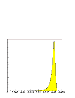
Figure 5: The ring radius distribution (horizontal axis in radians) used in the LHbC RICH simulation of Section 10. The functional form is shown in Equation 4.

7 Results

(a) event 1

(b) event 2

(c) event 3

(d) event 4

(e) event 5

(f) event 6

(g) event 7

(h) event 8

Figure 6: Fit performance allowing three seconds per event on a 3 GHz Pentium 4 computer. In each event, the result of the fit (i.e. the sample taken 3 seconds after sampling began) is shown on the left, while the “true” distribution of rings which generated the hits is shown on the right. All results are shown in a hyperbolic projection which compresses the whole of 2-space onto a disc. This projection is the cause of the elliptic distortion at the periphery of the disc.

Figure 6 shows the fits obtained after three seconds of sampling (each) for eight events on a 3 GHz Pentium 4 computer. No special selection was applied to these events. They are just the first eight events generated according to the toy model of Section 10. Note that in the time alotted the ring-finder missed a ring in event 6, and fitted a ring in event 7 poorly (the ring third from the bottom). All other rings are fitted well. The lowest ring multiplicity observed in the eight events was 3 rings in event 1. Event 5 had the most rings: 15.

More work needs to be done to optimise the termination criterion for the sampling process. Just stopping each event after three seconds or a fixed number of samples is very crude. A more sensible stopping criterion might choose to run complicated events (events with a large number of hits) for longer than simple ones. Even though better stopping criteria may be found in the future, it is clear from the very simple one implemented here that the ring-finder is indeed able to find rings.

8 Conclusions

This article has described an algorithm optimised for identifying rings among photons in RICH detectors which are similar to the LHbC RICH toy model of Section 10.

The algorithm acts only on hits, and does not have to be seeded with the locations of, for example, the centres of the rings.

The algorithm has demonstrated good performace on events produced by the toy model described in the text, at a cost of 3-seconds per event on a 3 GHz Pentium 4.

There is ample scope to optimise the ring-finder further, by finding better proposal functions and more realistic detector models.

9 Acknowledgements

The author would like to thank Dr. C. R. Jones for his continued support throughout the development of the ring-finder, and for his comments on the draft document. This work was partly funded by the author’s Particle Physics and Astronomy Research Council (PPARC) Fellowship.

10 Appendix: Details of Lester’s Highly basic Computational (LHbC) RICH simulation

This section lists the constituents of the toy model assumed for hit-production in order to calculate explicit forms for $p_{P}({\bf H}|{\bf R})$ and $p_{M}({\bf R})$ introduced in Section 4. The same model was used to generate the events shown in Figure 6 which were subsequently fitted by the ring-finder. It is hoped that the particular distributions and numbers chosen to define Lester’s Highly basic Computational (LHbC) RICH simulation will make the events it generates similar to those which might be seen in a future RICH detector of some kind.

The number of rings in an event was taken to be Poisson distributed with mean 10. The radius of each ring was assumed to be distributed according to a probability distribution proportional to the parameterization:

$${e^{625(x-0.0305)}}\over{(1+e^{5(x-0.0305)})(1+e^{2941(x-0.0305)})}$$ (4)

(for $x$ measured in radians) which is shown in Figure 5. The $x$ and $y$ co-ordinates of the centre of each ring were taken to be independent and Gaussian distributed with mean 0 and standard deviation 0.09 radians. (All distance values are measured in radians as we work in angular co-ordinates.) The mean number of hits per unit length $\rho$ on the circumference of each ring was 30/radian. The actual number of hits on a ring with radius $r_{R}$ was Poisson distributed with mean $2\pi r_{R}\rho$. The hits themseleves were taken to be distributed uniformly in azimuthal angle $\phi$, and with radii $r_{h}$ (distance from centre of ring) distributed independently for each hit according to

$$p({{r_{h}}|{r_{R}},{\epsilon},{\alpha}}) \propto \frac{1}{2\pi{r_{h}}^{2}}({\frac{{r_{h}}}{{r_{R}}}})^{{\alpha}-2}\exp(-\frac{\log^{2}\!({r_{h}}/{r_{R}})}{2{\epsilon}^{2}})$$ (5)

in which the dimensionless parameter ${\alpha}$ controlling the distribution skew took the value 2, and in which the dimensionless parameter ${\epsilon}$ controlling the thikness of the ring took the value 0.05.

The number of background hits (hits not coming from Cherenkov photons) in an event was taken to be Poisson distributed with mean 10. The $x$ and $y$ co-ordinates of each background hit were taken to be independently distributed acoording to the same Gaussian distributions used for the $x$ and $y$ co-ordinates of ring centres.

References

-
[1]
S. Amato, et al., LHCb technical proposal CERN-LHCC-98-4.
URL http://weblib.cern.ch/abstract?CERN-LHCC-P-4 -
[2]
LHCb: RICH technical design report. ISBN 92-9083-170-7 CERN-LHCC-2000-037.
URL http://lhcb.web.cern.ch/lhcb/TDR/TDR.htm - [3] A. Linka, J. Picek, P. Volf, G. Ososkov, New solution to circle fitting problem in analysis of RICH detector data, Czech. J. Phys. 49S2 (1999) 161–168.
- [4] D. Elia, et al., A pattern recognition method for the RICH-based HMPID detector in ALICE, Nucl. Instrum. Meth. A433 (1999) 262–267.
- [5] D. Cozza, D. Di Bari, D. Elia, E. Nappi, A. Di Mauro, A. Morsch, G. Paic, F. Piuz, Recognition of Cherenkov patterns in high multiplicity environments, Nucl. Instrum. Meth. A482 (2002) 226–237.
- [6] D. Di Bari, The pattern recognition method for the CsI-RICH detector in ALICE, Nucl. Instrum. Meth. A502 (2003) 300–304.
- [7] D. Ioannou, W. Huda, A. Laine, Circle recognition through a 2D Hough transform and radius histogramming, Image and Vision Computing 17 (1) (1999) 27–36.
- [8] J.-P. Andreu, A. Rinnhofer, Enhancement of annual rings on industrial CT images of logs. 3 (2002) 30261–30276, proceedings of the 16th International Conference on Pattern Recognition (ICPR’02) Volume 3.
-
[9]
LHCb Colaboration, LHCb Technical Design Report: Reoptimized detector
design and performance. ISBN 92-9083-209-6, CERN-LHCC-2003-030.
URL http://cdsweb.cern.ch/search.py?sysno=002388295CER - [10] D. J. M. MacKay, Information Theory, Inference, and Learning Algorithms, Cambridge University Press, 2003.
- [11] N. Metropolis, A. Rosenbluth, M. Rosenbluth, A. Teller, E. Teller, Equations of state calculations by fast computing machines, Journal of Chemical Physics 21 (1953) 1087–1091.
- [12] W. Hastings, Monte Carlo sampling methods using markov chains and their applications, Biometrika 57 (1970) 97–109.
- [13] Dr C.R. Jones, Cavendish Laboratory, University of Cambridge, UK. Private Communication.
- [14] Dr C.G. Lester and Dr C.R. Jones (in preparation).
- [15] A. G. Buckley, A study of decays with the LHCb experiment, Ph.D. thesis, University of Cambridge, Cavendish Laboratory, (in preparation) (2005).