Non-transitive maps in phase synchronization

Abstract

Concepts from Ergodic Theory are used to describe the existence of special non-transitive maps in attractors of phase synchronous chaotic oscillators. In particular, it is shown that for a class of phase-coherent oscillators, these special maps imply phase synchronization. We illustrate these ideas in the sinusoidally forced Chua’s circuit and two coupled Rössler oscillators. Furthermore, these results are extended to other coupled chaotic systems. In addition, a phase for a chaotic attractor is defined from the tangent vector of the flow. Finally, it is discussed how these maps can be used to a real-time detection of phase synchronization in experimental systems.

1 Introduction

Coupled chaotic systems are recently calling much attention due to the verification that they may be useful to the understanding of natural systems in a variety of fields as in ecology [1], in neuroscience [2, 3], in economy [4], and in lasers [5, 6]. It has been verified that despite of the higher dimensionality of a coupled chaotic system, the coupling among the elements might make them to synchronize [7, 8], reducing the dynamics of the system to a few degrees of freedom.

In this work, we focus our attention in the phenomenon of Phase Synchronization (PS), which describes the appearance of a phase synchronous behavior between two interacting chaotic systems [9], i.e., given two chaotic systems, their phase difference remains bounded, despite of the fact that their amplitudes may be uncorrelated. This phenomenon is particularly interesting since it can arise from a very small coupling strength. Its presence was reported in a variety of experimental systems. It was experimentally demonstrated in electronic circuits [10], and latter in electrochemical oscillators [11]. It was found in plasma [12], in the Chua’s circuit [13], and there were also found evidences of phase synchronization in communication processes in the Human brain [14, 15] .

To detect PS in a real-time experiment, one has to measure the phase of the chaotic trajectory [16]. However, the phase is not always an easily accessible information. To overcome this difficulty, it is important to understand fundamental properties of phase synchronous systems, that could be experimentally easily verified. For chaotic systems that are phase synchronized with a periodic forcing [17], it was reported that a stroboscopic map of the trajectory was a subset of this attractor and occupies only partially the region delimitated by a projection of the attractor. This property was used to detect in a real-time experiment phase synchronization between the Chua’s circuit and a sinusoidal forcing [13].

This approach of detecting phase synchronization through the stroboscopic map can be extended for coupled chaotic oscillators, in a formal way. The stroboscopic map is generalized to the Conditional Poincaré Map. Given two oscillators, at least one being chaotic, the conditional Poincaré map is constructed by collecting points in one oscillator at the moment at which some event happens in the other one. If the set of discrete points generated by this conditional map does not visit any arbitrary region of a especial projection of the chaotic attractor, we call this set a P-set. This property of the conditional Poincaré map is called non-transitivity [18], i.e., an initial condition under the conditional Poincaré map does not visit everywhere in a subspace of the attractor. Alike the stroboscopic maps of oscillators that are in phase synchrony with a forcing, the conditional Poincaré maps of coupled chaotic oscillators, in PS, also only partially occupy a projection of the attractor.

In this work, we show how the conditional Poincaré map can be used to detect PS, without actually having to measure the phase. For phase-coherent oscillators, a special type of P-set, that we call PS-set (Phase Synchronization set), exists. Conversely, its existence also implies PS. We illustrate our findings and ideas with numerical and experimental analyzes in the forced Chua’s circuit, and the coupled Rösller oscillator [19].

Further, we extend these results to non-phase coherent attractors. Finally, we also introduce a phase of a chaotic trajectory to be a quantity related to the amount of rotation of the tangent vector. This definition can be used to chaotic attractors, independently whether they have phase-coherent or non phase-coherent dynamics.

This work is organized as follows: in Sec. 2, we define a way to measure the phase of a chaotic flow, and discuss the relation between the average returning time and the average angular frequency. In Sec. 3, we discuss the conditions for PS states and, in Sec. 4, we describe the phenomenon of PS in the forced Chua’s Circuit. We introduce the notion of a conditional Poincaré map in Sec. 5 and the P-sets (as well as the PS-sets) in Sec. 6. In Sec. 7, we show how PS can be found by the detection of these sets in the forced Chua’s Circuit and in Sec. 8, for the coupled Rössler oscillator. Further, in Sec. 9, we discuss the extension of these ideas to a class of non-coherent oscillators. In Sec. 10, we make some remarks and the conclusions of this work. In Appendix A, we formally introduce the conditional Poincaré map and the P-set, and in Appendix B, we show that for coherent dynamics the PS-sets exist if, and only if, there is PS. In other words, PS implies PS-sets and vice-versa.

2 Phase, frequency and average returning time of a chaotic attractor

The phase of a chaotic attractor in a projection $j$ (a subspace) is defined to be the amount of rotation of the tangent vector in this projection, and can be represented by an integral function of the type

$$\phi_{j}(t)=\int_{0}^{t}\left|\frac{d\theta(t^{{}^{\prime}})}{dt^{{}^{\prime}}}\right|dt^{{}^{\prime}}$$ (1)

with $d\theta(t)$ being an infinitesimal displacement of the tangent vector of the flow, from time $t$ to time $t+dt$, and $dt\rightarrow 0$. Note that in Eq. (1), we are measuring the amount of rotation, per unit time, of a projection of the tangent vector of the flow, on the same subspace $j$ where the phase is defined. We call this subspace $\mathcal{P}_{j}$. The attractor $\mathcal{X}$, projected on the subspace $\mathcal{P}_{j}$ is regarded as $\mathcal{X}_{j}$. The instantaneous angular frequency of the trajectory in $\mathcal{X}_{j}$, named $W_{j}$ is given by $\frac{d\phi_{j}}{dt}$. So, from Eq. (1), $W_{j}=\left|\frac{d\theta}{dt}\right|$ and, the average angular frequency $\langle W_{j}\rangle$ is

$$\langle W_{j}\rangle=\lim_{t\rightarrow\infty}\langle\frac{d\phi_{j}}{dt}\rangle,$$ (2)

$\langle-\rangle$ represents the average. Equation (2) can be put into the form $\langle W_{j}\rangle$ = $\frac{\phi_{j}(t)}{t}$.

Whenever a Poincaré section can be defined, the average period of the chaotic attractor on the subspace $\mathcal{P}_{j}$ is calculated by

$$\langle T_{j}\rangle=\frac{\sum_{i=0}^{N}\Delta\tau^{i}_{j}}{N},$$ (3)

where $\Delta\tau^{i}_{j}=\tau^{i}_{j}-\tau^{i-1}_{j}$, and $\tau^{i}_{j}$ represents the time at which the trajectory in the subspace $\mathcal{P}_{j}$ makes the $i$-th crossing with this Poincaré section.

We introduce $\langle\Delta\phi_{j}\rangle$ to be the average displacement of the phase for a typical period as

$$\langle\Delta\phi_{j}\rangle=\frac{\phi_{j}(N)}{N},$$ (4)

with $\phi_{j}(N)$ being the phase associated to the subspace $\mathcal{P}_{j}$ at the moment that the $N$-th crossing between the trajectory and the Poincaré section happens.

Thus, we can put Eq. (2) as

$$\langle W_{j}\rangle=\frac{\langle\Delta\phi_{j}\rangle}{\langle T_{j}\rangle}.$$ (5)

For the forced Chua’s circuit, the subspace $\mathcal{P}_{1}$ is defined by a suitable projection of the circuit variable. We have that $\langle\Delta\phi_{1}\rangle=2\pi$. So, Eq. (5) can be written as $\langle W_{1}\rangle=\frac{2\pi}{\langle T_{1}\rangle}$. For the coupled Rössler oscillator, the quantities in Eq. (5) can be calculated in two subspaces, one associated to the variables of one Rössler, the subspace $\mathcal{P}_{1}$, and the subspace $\mathcal{P}_{2}$, associated to the variables of the other Rössler system. As shown in [21], $\langle\Delta\phi_{1}\rangle$ might slightly differs from $2\pi$, and thus, $\langle W_{j}\rangle=\frac{\langle\Delta\phi_{j}\rangle}{\langle T_{j}\rangle}$.

So, Eqs. (2) and (5) relate the average period, the average angular frequency, and the phase of a chaotic trajectory. This shows that the average period (recurrence) and the average angular frequency are intimately connected in phase coherent chaotic systems, and both these quantities can be calculated from the phase.

3 Phase Synchronization

Having defined phase, PS exists whenever the following condition is satisfied

$$|\phi_{1}(t)-r\phi_{2}(t)|<\langle\Delta\phi_{1}\rangle.$$ (6)

The minimal bound for the phase difference, $\langle\Delta\phi_{1}\rangle$, in terms of the phase as defined by Eq. (6), was theoretically estimated in Ref. [21]. Equation (6) means that the phase difference between the two coupled systems is always bounded, and $r$ is a rational constant [22].

Also,

$$\langle W_{1}\rangle-r\langle W_{2}\rangle=0.$$ (7)

In this work, we will consider cases for $r$=1. Otherwise, a simple change of variables could eliminate this constant from Eq. (7). For the forced Chua’s circuit $\langle W_{2}\rangle=\omega$, with $\omega=2\pi f$, representing the angular frequency of the forcing. There is PS, if $\langle W_{1}\rangle$=$\omega$. Therefore, $\langle T_{1}\rangle$=$1/f$. For the coupled Rössler, if PS exists, $\langle W_{1}\rangle$ = $\langle W_{2}\rangle$, $\langle R_{1}\rangle$=$\langle R_{2}\rangle$, and $\langle\Delta\phi_{1}\rangle$=$\langle\Delta\phi_{2}\rangle$, and therefore, we could have in the right term of Eq. (6) $\langle\Delta\phi_{2}\rangle$, instead of $\langle\Delta\phi_{1}\rangle$.

4 The sinusoidally forced Chua’s circuit

The circuit is represented by:

$$C_{1}\frac{dX_{1}}{dt}=g(X_{2}-X_{1})-i_{NL}$$ (8)

$$C_{2}\frac{dX_{2}}{dt}=g(X_{1}-X_{2})+X_{3}$$ (9)

$$L\frac{dX_{3}}{dt}=-X_{2}-V\sin{(\omega t)}$$ (10)

where $X_{1}$, $X_{2}$, and $X_{3}$ represent, respectively, the tension across two capacitors and the current through the inductor (See [13] for more details), $\omega$ and $V$ are the angular frequency and the amplitude of the forcing, respectively. The piecewise-linear function, $i_{NL}$, is given by:

$$i_{NL}=m_{0}X_{1}+0.5(m_{1}-m_{0})[|X_{1}+B_{p}|-|X_{1}-B_{p}|]$$ (11)

where we have chosen the parameters $C_{1}$=0.1, $g$=0.574, $C_{2}$=1, $L$=1/6, $m_{0}$=-0.5, and $m_{1}$=-0.8, such that we obtain a Rössler-type attractor, for $V$=0.

To calculate the phase of the chaotic trajectory, we first define the subspace $\mathcal{P}_{1}$ to be given by the pair of variables $(X_{1},X_{2})$, and then, we use Eq. (1). In Fig. 1, we show the difference between the phase of the chaotic circuit [as calculated by Eq. (1)] and the phase of the forcing, $\omega t$. In (a), the phase difference is bounded and the average period of the chaotic attractor, defined as the average recurrence time of trajectories that cross the section $X_{2}=0$, is equal to $\langle T_{1}\rangle$=3.57015, which is equal to 1/f, since $f$=0.2801. The average angular frequency can be calculated using Eq. (5), which gives us $\langle W_{1}\rangle$=1.75992. Or, from Eq. (2), which gives us $\langle W_{1}\rangle$=1.75992. Note that the average growing of the phase [calculated by Eq. (1)] for a typical average period is $6.28318\ldots$ which is $2\pi$. In Fig. 1(b), we have that $\langle T_{1}\rangle$=3.57006 which is different from $1/f$, since $f$=0.279. So, in (b) there is no PS, and consequently Inequality (6) is not satisfied.

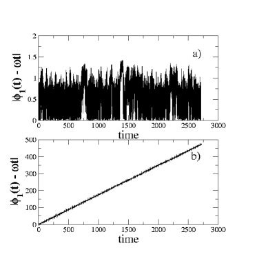
Figure 1: (a) Phase difference is always smaller than 2$\pi$, so PS exists between the circuit and the forcing, for $f$=0.2801 and $V$=0.0015. (b) PS is not present and the phase difference grows bigger than 2$\pi$.

In Ref. [13], we detected $PS$ experimentally in the forced Chua’s circuit, whenever stroboscopic maps could be constructed for a time interval equal to $\Delta\tau_{1}=\frac{1}{f}$, such that this map, projected into the same subspace considered to calculate the phase, does not occupy the region occupied by the attractor projected on the same subspace.

To understand this technique, we assume that $\phi_{1}(t)$, the phase of the chaotic trajectory, is the angle (on the lift) described by the vector position of this trajectory (Rössler-Like attractor), and $\phi_{2}(t)$=$\omega t$ the phase of the forcing. If Eq. (6) is satisfied at any time, then it is satisfied at multiples of the period of the forcing $\tau_{1}^{i}=\frac{i}{f}$. So, we get $|\phi_{1}(\tau_{1}^{i})-2\pi i|<2\pi$, which means that a stroboscopic map has to be concentrated in an angular section smaller than $2\pi$. The stroboscopic map, which is already a subset of the chaotic flow, projected into the same subspace considered to calculate the phase, does not occupy the whole region occupied by the attractor projected in this same subspace. Another property of the stroboscopic map is that points in it are mapped into it by looking at the trajectory after a time interval given by $\Delta\tau_{1}$, so, it is a subset that is recurrent to itself.

Using this technique, and for the same parameters as [13], we show in Fig. 2(a) the experimental synchronization region for the forced Chua’s circuit in the parameter space $V\times f$. The triangular shaped region represents parameters for which the stroboscopic map has the points concentrated in an angular section smaller than 2$\pi$. The bump at the bottom right side of the PS region is due to non-synchronous states that present a long bounded phase difference. By a typical time interval within which the experiment is realized, which was of the order of 40,000 cycles, the system seemed to be phase synchronized, i.e., localized stroboscopic maps were found. In fact, we have detected these maps even for observation times corresponding to 150,000 cycles, in the region of the bump.

In a short, the bump region is an extended structure in the circuit parameter space, that presents intermittent behavior in the phase difference [24], but with a long laminar regime, even for parameters far away from the border between the PS and the non PS region. This intermittency differs from the usual one, observed in the transition to PS, in the fact that this latter happens very close to the border between the PS and the non PS region. The reason for this intermittency is due to the presence of a periodic window, close to the region of the bump.

Simulation is shown in Fig. 2(b), where black points represent perturbing parameters for which Eq. (6) is satisfied, with $\phi_{1}$ defined in Eq. (1). One sees that the $PS$ region resembles a triangle. The triangular shaped region, denoted by the light gray dashed line, represents the region where the system is not phase synchronized, but the phase difference remains bounded for a long time interval, that might be longer than 100,000 cycles of the systems. So, we reproduce numerically the same atypical intermittency observed experimentally, i.e., long laminar regime in the phase difference, for parameter regions away from the border between PS and non PS states. This happens associated with a periodic window, as the one shown in Fig. 2(b).

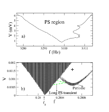
Figure 2: (a) Experimental $PS$ parameter space. (b) Simulated $PS$ parameter space. Black points represent parameters for which Eq. (6) is satisfied for 120,000 crossings of the trajectory at $X_{2}$=0. In both figures, the horizontal axis represents the forcing frequency $f$ and the vertical axis its amplitude $V$. Variables in (b) are dimensionless and $f_{0}$ is the main frequency of the non-forced circuit.

The shape of the synchronization region in Fig. 2(b) is equivalent to the region in the experiment, constructed by detecting the stroboscopic maps contained within a small angular section. This proposes an equivalence between the existence of a recurrent subset and the verification of Eq. (6). Inside the synchronization region, a stroboscopic map appears like in Fig. 3(a), where the light gray points represent the attractor, and the dark filled circles, the map. Outside of the $PS$ region, there are parameter sets for which the stroboscopic maps do not occupy the region occupied by the attractor, at the projection in which the phase is calculated. As one sees in Fig. 3(b) [for the parameters represented by the plus symbol in Fig. 2(b)] there is a region of the projected attractor (pointed by the arrow) for which the stroboscopic map never visits.

The difference between the stroboscopic map that appears while there is PS in (a), and the stroboscopic map that appears while there is not PS in (b), is that points of the stroboscopic map in (a) are all concentrated in an angular section of the attractor. As it will be further classified, the stroboscopic map in (a) is a PS-set and in (b) is a P-set.

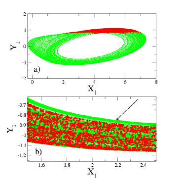
Figure 3: A projection of the attractor in light gray, and its stroboscopic map in dark gray. The parameters are $f$=0.2801 and $V$=0.0015, in (a), and $f$=0.28063 and $V$=0.0016, in (b).

As a way to better characterize the PS phenomena in the Chua’s circuit, we calculate the Lyapunov exponents. As usually expected, the transition to PS is associated to one of the exponents becoming smaller than zero. Since there is already one exponent that is smaller than zero, PS induces the creation of a second stable direction in the Chua’s circuit. Previous to the transition to phase synchronization, this exponent was zero. In Fig. 4, we show the exponent (and the error bars) associated to PS in black and the quantity $\langle W_{1}\rangle-\omega$ (in gray, for a fixed amplitude of $V$=0.0015) with respect to the frequency. In the region that the exponent becomes smaller than zero, $\langle W_{1}\rangle$=$\omega$, satisfying Eq. (7).

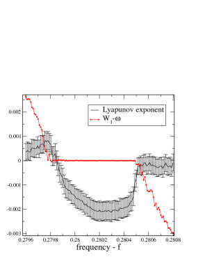
Figure 4: The Lyapunov exponent (and the error bars) associated to PS in black, and the quantity $\langle W_{1}\rangle-\omega$ in gray, for a fixed amplitude of $V$=0.0015 and a varying frequency.

5 Conditional Poincaré Map

The finding of maps of the attractor that appear as localized structures implies PS. The conditional Poincaré map introduced in this chapter as a generalization of the stroboscopic map, is an efficient way of revealing the existence of such special mappings.

The stroboscopic map technique defined for periodically driven chaotic systems was explained in the previous sections. To extent the idea of stroboscopic map in coupled chaotic oscillators we came up with the conditional Poincaré map, which is a map of the flow, constructed by observing it for specific times at which events occur in the subsystems $\mathcal{X}_{j}$. An event is considered to happen when the trajectory of one subsystem crosses a Poincaré section. So, given two oscillators $S_{1}$ and $S_{2}$ (at least one being chaotic), with trajectories in the subspaces where the phase is defined, the conditional Poincaré map of $S_{1}$ is the trajectory position at the moment that a series of equal events happens, in $S_{2}$. Analogously, the conditional Poincaré map of $S_{2}$ is the trajectory position at the moment that a series of equal events happens, in $S_{1}$. In the case of periodically forced chaotic systems, an event may be defined to happen whenever the forcing reaches a specific value, and the conditional Poincaré map is the usual stroboscopic map, because the time interval between two events is constant. In coupled chaotic systems, the time interval between two successive events is no longer constant.

We define a time series of events $\tau^{i}_{j}$, by the following rule:

• $\tau^{i}_{1}$ represents the time at which the $i$-th crossing of the trajectory of $S_{2}$ occurs in a Poincaré plane.

• $\tau^{i}_{2}$ represents the time at which the $i$-th crossing of the trajectory of $S_{1}$ occurs in a Poincaré plane.

The discrete set of points observed at the times $\tau^{i}_{j}$ is called set $\mathcal{D}$. This set, projected at the subspaces $\mathcal{P}_{j}$ (where the phase is calculated), is named $\mathcal{D}_{j}$. The conditional Poincaré map is represented by $T^{\tau_{j}^{i}}$. So, we say that $\mathcal{D}_{j}$ is the set of points generated by $T^{\tau_{j}^{i}}$.

The next step is to define when $\mathcal{D}_{j}$ can be regarded as either a P-set or a PS-set, this last set implying phase synchronization.

6 Sets generated by the Conditional Poincaré Map

The $\mathcal{D}_{j}$ set is a P-set, if it does not completely fulfill the projection $\mathcal{X}_{j}$ of the attractor. In other words, a discrete set $\mathcal{D}_{j}$ is considered to be a P-set, if for balls of radius $\delta$, centered in all points of the attractor projection $\mathcal{X}_{j}$, one does not find points of $\mathcal{D}_{j}$ inside of all these balls. If $\mathcal{D}_{j}$ completely fulfill $\mathcal{X}_{j}$, we say that these two sets are equivalent (and we represent this by the symbol $\equiv$). More details, see Appendix A.

So, a P-set exists, if the conditional Poincaré map is not transitive on $\mathcal{X}_{j}$ [18]. That is, the flow, observed by the times for which the conditional Poincaré map is defined, does not visit arbitrary regions of $\mathcal{X}_{j}$. Note that however, the attractor is chaotic, and therefore, the chaotic set is always transitive through the flow. So, given a set of initial conditions, its evolution through the flow eventually reaches arbitrary open subsets of the original chaotic attractor.

We can classify three relevant types of sets generated by the conditional Poincaré map

type-a

$\mathcal{D}_{j}$ is equivalent to $\mathcal{X}_{j}$ ($\mathcal{D}_{j}\equiv\mathcal{X}_{j}$). The conditional Poincaré map $T^{\tau_{j}^{i}}$ is transitive in $\mathcal{X}_{j}$.

P-set

$\mathcal{D}_{j}$ is NOT equivalent to $\mathcal{X}_{j}$ ($\mathcal{D}_{j}\not\equiv\mathcal{X}_{j}$). The conditional Poincaré map is NOT transitive in $\mathcal{X}_{j}$.

PS-set

$\mathcal{D}_{j}$ is P-set, with the additional condition that it is localized in the vicinity of the Poincaré section chosen to define the events.

In the following, we comment each case:

6.1 type-a sets

These sets appear whenever there is no PS. If two non-identical coupled chaotic systems (topologically similar) are not phase synchronized, the chaotic trajectories do not make correlated events in both subspaces $\mathcal{P}_{1}$ and $\mathcal{P}_{2}$. As a consequence while the trajectory is positioned at the specified Poincaré plane, at the subspace $\mathcal{P}_{1}$, the trajectory in the subspace $\mathcal{P}_{2}$ is everywhere in this subspace, making the set $\mathcal{D}_{j}$ to be equivalent to $\mathcal{X}_{j}$.

An interesting illustration is the case of two uncoupled equal chaotic systems, but with different initial conditions. As we construct the conditional Poincaré maps, they will be a type-a set, since also the distance between the trajectories in the two oscillators are sensitive to the initial conditions, and will diverge exponentially.

6.2 P-sets

These sets constitutes a necessary, but not sufficient, condition to describe PS.

In periodically forced chaotic systems, they might appear when there is not PS. As we already mentioned, the points in these sets are not localized in special spots of the attractor projection. As a consequence, the domain of the absolute difference between the time at which the same number of events happen in both oscillators has a broad character.

6.3 PS-sets

PS-sets imply PS and vice-versa. They exist, if and only if, there is phase synchronization, as shown in Appendix B, and illustrated with the examples in Sec. 4, and throughout this work. Another important point is that the PS-set provides a real-time detection that can be easily experimentally implemented (Sec. 4), and easily constructed from a data set.

PS-set implies PS because the difference between the time at which the $N$-th event happens in both oscillators is small, which means that the time difference $|\tau_{1}^{N}-\tau_{2}^{N}|$ is smaller than a finite constant value. As a consequence, the points in the conditional Poincaré map of one oscillator are confined around the Poincaré section chosen to define the events. Therefore, the detection of a PS-set can be done by observing this characteristic of the conditional Poincaré map.

For Rössler-like oscillators, in which the trajectory spirals around an equilibrium point, the PS-set is confined within an angular section.

6.4 Length of a PS-set

Having found the PS-set, we can study properties of these sets that give us the level of organization and coherence of the oscillators

A PS-set, $\mathcal{D}_{j}$, is said to have length 1, if the set is constructed by the time series of the same events. Defining the event to be given by the crossing of the trajectory to a Poincaré plane, the corresponding time series of events $M_{j}(1)$ is given by $\tau_{j}^{i},\tau_{j}^{i+1},\tau_{j}^{i+2},\tau_{j}^{i+3},\ldots$. For this PS-set, points in $\mathcal{D}_{j}$ are mapped in $\mathcal{D}_{j}$, after one application of the conditional Poincaré map.

A PS-set is said to have length 2, if it is obtained by a time series of two different events. So, a PS-set can be constructed from more complex series of events. We construct a length-2 basic set using a time series of events $M_{j}(2)$ given by $\tau_{j}^{i},\frac{\tau_{j}^{i}+\tau_{j}^{i+1}}{2},\tau_{j}^{i+1},\frac{\tau_{j}^{i+1}+\tau_{j}^{i+2}}{2},\ldots$ [25]. As an example, for the perturbed Chua’s circuit, the length-2 basic set is constructed by a stroboscopic map that collects points every half period of the forcing. A length-2 basic set is assumed to be composed by two other subsets, named minimal sets, the subsets $\mathcal{D}_{j}^{0}$ and $\mathcal{D}_{j}^{1}$.

They have the property that if a point $x_{0}$ is such that $x_{0}\in\mathcal{D}_{j}^{0}$, this point, iterated by the conditional Poincaré map, goes to the minimal set $\mathcal{D}_{j}^{1}$, and if $x_{0}$ is such that $x_{0}\in\mathcal{D}_{j}^{1}$, this point, iterated by the conditional Poincaré map, goes to the minimal set $\mathcal{D}_{j}^{1}$. Thus, points in $\mathcal{D}_{j}^{1}$ are mapped to itself after 2 applications of the conditional Poincaré map. The minimal set $\mathcal{D}_{j}^{1}$ is said to be disjoint to the set $\mathcal{D}_{j}^{2}$, if they do not intersect, i.e., $\mathcal{D}_{j}^{1}\cap\mathcal{D}_{j}^{2}=\emptyset$. For some systems that present a strong phase-coherent state, as the ones here studied, in which the instantaneous trajectory velocity does not differ too much from the average velocity on typical orbits, it is possible to find length-2 basic set, with disjoint minimal sets, when PS is present.

For a general case, we do not expect to find a length-2 PS-set with disjoint minimal sets. As an example, one can think of a spiking-firing oscillator, phase synchronized with a periodic forcing. Due to the fact that the spiking-firing dynamics has a fast and a slow mode, the conditional Poincaré maps might overlap.

6.5 Sets diagram

Here, we explain through a diagram the possible emerging sets from the conditional Poincaré map.

Starting from the chaotic attractor $\mathcal{X}$, the set $\mathcal{D}$ is constructed from the conditional Poincaré map, represented by $T$, we project $\mathcal{D}$ and $\mathcal{X}$ into the subspace $\mathcal{P}_{j}$, obtaining the sets $\mathcal{D}_{j}$ and $\mathcal{X}_{j}$, respectively.

We classify the set $\mathcal{D}_{j}$ into type-a set or P-set, by checking whether the conditional Poincaré map is transitive in $\mathcal{X}_{j}$, i.e., by verifying the equivalence between the sets $\mathcal{X}_{j}$ and $\mathcal{D}_{j}$. Then, if the P-set is localized in the vicinity of the Poincaré section where the events occur, the P-set is a PS-set, which means that PS is present.

7 PS-sets in the Chua’s circuit

For applying our formalism to the periodically forced Chua’s circuit, the event times are $\tau_{1}^{i}=i\tau$, with $\tau$ representing the forcing period. The time series for the length-2 basic set is given by ${1/2\tau,\tau,3/2\tau,2\tau,5/2\tau,3\tau,\ldots}$. Everywhere inside the $PS$ region, we find length-1 [as an example, see Fig. 3(a)] and length-2 [as an example, see Fig. 5(a)] PS-sets, this latter with disjoint minimal sets. In Fig. 5(a), the application of the conditional Poincaré map in the minimal set $\mathcal{D}_{1}^{0}$ leads to the minimal set $\mathcal{D}_{1}^{1}$. Both sets form a length-2 PS-set. Note that both $\mathcal{D}_{1}^{0}$ and $\mathcal{D}_{1}^{1}$ can be regarded as a length-1 PS-set. To our numerical precision, we have checked that there are not basic sets beneath the Synchronization region tip. Which means that type-a set is present for very small but finite amplitude forcing. Outside the $PS$ region, there is a P-set, i.e., a non-transitive conditional Poincaré map on the chaotic attractor projection. So, $\mathcal{D}_{j}\not\equiv\mathcal{X}_{j}$. In this case, there is not PS. More examples of length-Q PS-sets in the phase synchronous forced Chua’s circuit can be seen in [26].

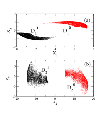
Figure 5: (a) Length-2 PS-set with disjoint minimal sets, in the forced Chua’s circuit, for the parameters $f$ = 0.2801 and $V$ = 0.001. The PS-set is constructed by the time series $M_{1}(2)$. (b) Length-2 PS-set with disjoint minimal sets, in the coupled Rössler oscillators, for the parameters $\epsilon$=0.01 and $\delta\alpha$ = 0.001. The PS-set is constructed by the time series $M_{2}(2)$.

8 PS-sets in the coupled Rössler system

We can use the formalism of the conditional Poincaré map to study the appearance of PS in coupled chaotic systems, as the two coupled Rössler oscillators given by:

$$\dot{x}_{1,2}=-\alpha_{1,2}y_{1}-z_{1}+\epsilon(x_{2,1}-x_{1,2})$$ (12)

$$\dot{y}_{1,2}=\alpha_{1,2}x_{1}+0.15y_{1}$$ (13)

$$\dot{z}_{1,2}=0.2+z_{1}(x_{1}-10)$$ (14)

with $\alpha_{1}=1$, and $\alpha_{2}=\alpha_{1}+\delta\alpha$. The index denotes systems 1 and 2. The subspaces $\mathcal{P}_{j}$ are defined by $\mathcal{P}_{j}$=$(x_{j},y_{j})$. In a coupled chaotic system, $\tau_{1}^{i}$ ($\tau_{2}^{i}$) does not increase uniformly, but it is given by the time the trajectory crosses the Poincaré plane $y_{2}$=0 ($y_{1}$=0). For these times, and using the time series $M_{j}(2)$, we construct the minimal sets $\mathcal{D}_{1}^{0}$ and $\mathcal{D}_{1}^{1}$ ($\mathcal{D}_{2}^{0}$ and $\mathcal{D}_{2}^{1}$). The parameters are $\epsilon$=0.01 and $\delta\alpha$ = 0.001.

In Fig. 5(b), we show a length-2 basic set with disjoint minimal sets. The application of the conditional Poincaré map in the minimal set $\mathcal{D}_{2}^{0}$ leads to the minimal set $\mathcal{D}_{2}^{1}$, and vice-versa. These two sets form together a length-2 PS-set, but each one separated can be regarded as a length-1 PS-set. The characteristic of these PS-sets is that they appear as localized structures around the Poincaré section chosen to define the events. As one can see, the set $\mathcal{D}_{2}^{0}$ is localized in the neighborhood of the line $y_{2}=0$, where the Poincaré section is chosen.

In fact, this length-2 PS-set with disjoint minimal sets (as well as a length-1 PS-set) is found everywhere in the PS region, as shown in Fig. 6. In it, filled squares represent parameters for which these special PS-sets are found, and empty circles parameters for which PS exists.

A PS-set of length-Q is detected using in Eq. (16) $\mathcal{D}_{2}^{Q-1}$, from which we can check whether $\mathcal{D}_{2}^{Q}$ occupies (type-a discrete set $\mathcal{D}$) the whole space occupied by $\mathcal{X}_{1}$. The set $B_{\ell}(x)$ in Eq. (16) is constructed assuming squares of size $\ell=1.5$, in points of the set $\mathcal{D}_{2}^{Q-1}$. In Fig. 6, we show a case for $Q$=2.

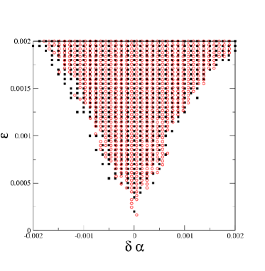
Figure 6: Empty circles show parameters for which PS exists, detected by Eq. (6), and filled squares represent parameters for which a length-1 PS-set appears simultaneously with a length-2 PS-set with disjoint minimal sets. Horizontal axis represents parameter mismatch and vertical axis, the coupling amplitude.

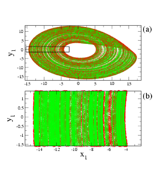
Figure 7: We show a situation where PS is not found for $\epsilon$=0.01 and $\delta\alpha$ = 0.00001. In (a), we show the attractor in the subspace $\mathcal{P}_{1}$, the subset $\mathcal{X}_{1}$ in gray, and the discrete set $\mathcal{D}_{1}$ in dark empty circles. In this figure, $\mathcal{D}_{1}$ is a type-a set, since $\mathcal{X}_{1}$ visits every neighborhood of points in $\mathcal{D}_{1}$ (the conditional Poincaré map is transitive in $\mathcal{X}_{1}$). In (b), we show a magnification of the box in (a).

In Fig. 7(a), we show the attractor in the subspace $\mathcal{P}_{1}$, the subset $\mathcal{X}_{1}$ in gray, and the discrete set $\mathcal{D}_{1}$ in dark empty circles . In (b), we show a magnification of the box in (a). Note that neighborhoods of arbitrary points in the trajectory of $\mathcal{X}_{1}$ (gray) always contain a point of the discrete set $\mathcal{D}_{1}$ (dark empty circles). So, the set $\mathcal{X}_{1}$ is equivalent to the set $\mathcal{D}_{1}$ and, therefore, $\mathcal{D}_{1}$ is not a PS-set, and therefore, it does not exist PS. Differently from the Chua’s circuit, the Rössler coupled system presents no P-sets for parameters outside of the PS region.

9 Extension to other coupled chaotic systems

The approach presented in this paper can be extended for non-coherent attractors. As noticed in Ref. [20], attractors that present non-coherent phase motion in the phase space may present a coherent motion in the space of the velocities, i.e. $(\dot{x},\dot{y})$, which is the case of the funnel attractor [20]. In this case, the extension of our approach to the non-coherent phase motion is straightforward. Instead of defining a conditional Poincaré map in the phase space, we analyze the dynamics in the velocity space, in which the phase is coherent, and therefore, all the ideas introduced herein can be applied in this new space.

To some chaotic attractors, it might not be possible to define a Poincaré section to construct the conditional Poincaré map. However, one can still construct these conditional maps by defining different types of events. For example, in coupled neurons, this event can be chosen as being a beginning or the ending of the bursts, which can be well defined by the crossing of the trajectory with some given threshold.

10 Conclusion and Remarks

A chaotic set is always transitive through the flow. So, given a set of initial conditions, its evolution through the flow eventually reaches arbitrary open subsets of the original chaotic attractor. However, a stroboscopic map of the flow, whose generalization is here called conditional Poincaré map, might not possess the transitive property. That is, given a set of initial conditions, its evolution through the conditional Poincaré map might not reach arbitrary open subsets of the chaotic attractor.

The introduction of the term “conditional” in the map nomenclature comes from the unconventional and non rigidly way we adapt the established definition of a stroboscopic Poincaré map. For coupled chaotic oscillators, this conditional map is constructed based on events, conveniently chosen at the same subspaces where the phase of a chaotic system is defined. In addition, the application of this map through the flow, which results in a discrete set, is inspected not in the whole phase space, but also in the same subspaces where the phase is defined.

If phase synchronization exists the conditional map generates special discrete sets, named PS-sets. The contrary is also true. i.e., a PS-set implies phase synchronization. This was illustrated in the periodically forced Chua’s circuit, in the coupled Rössler oscillator, and in other more general (topologically equivalent) coupled chaotic systems.

The ideas introduced here provide an efficient way of detecting phase synchronization, without having actually to measure the phase of the chaotic trajectory. Indeed, this detection can be done in experiments in a real-time, as it was done here in the perturbed Chua’s circuit.

It is worthy to say that the PS-sets are robust under small additive noise that could corrupt the data in an experiment. This is so, because a small additive noise does not interfere much with the time that the trajectory crosses the Poincaré section, but just deviates the timing of the crossing. Then, the PS-sets still remains. This robustness against the noise is an important property in order to apply these ideas in experiments, as done in this work.

We have also introduced the phase as a quantity that measures the velocity of rotation of a projection of the tangent vector along the trajectory. This definition can be used to arbitrary flows, independently whether or not they present a coherent or non-coherent phase dynamics.

Finally, our formalism of the conditional Poincaré map can be used in coupled maps (or perturbed) to detect synchronous behavior (not phase synchronization) between the systems (or between the forcing), for the case where one does not find full synchronization between the maps. One particular example where that happens is in the periodically forced Logistic equation [27] or for a system of coupled Logistic maps [28], where one can find a finite number of synchronous chaotic subsets, the basic sets.

Acknowledgment Research partially financed by FAPESP, Alexander Von Humboldt Foundation, and CNPq.

Appendix A The conditional Poincaré map and the $\mathcal{D}_{j}$ sets

Next, we present some formalism using elements of Ergodic Theory in order to introduce the conditional Poincaré map and the $\mathcal{D}_{j}$ sets.

Given a flow $F_{t}$, we call $\mathcal{X}$ the chaotic attractor. A subset of the attractor is its projection on the subspace $\mathcal{P}_{j}$, that we call $\mathcal{X}_{j}$. We assume $\mathcal{X}\in R^{d}$.

The notion of stroboscopic map of a flow can be generalized to any temporal translation on the trajectory. We define the temporal translation to be a transformation represented by $T^{\tau^{i}_{j}}$, called conditional Poincaré map. The initial condition $\vec{x}(t)$ is iterated under the temporal transformation $T^{\tau_{j}^{i}}$, to the point $\vec{x}(t+\tau_{j}^{i})$. Applying the transformation $T^{\tau_{j}^{i}}$ in a typical trajectory, for the time sequence $\tau_{j}^{i}$, $\tau_{j}^{i+1}$, $\tau_{j}^{i+2}$, give us the points $\vec{x}(\tau_{j}^{i})$, $\vec{x}(\tau_{j}^{i+1})$, and $\vec{x}(\tau_{j}^{i+2})$. So, $\vec{x}(\tau_{j}^{i+1})$ is the point $\vec{x}(\tau_{j}^{i})$ integrated by the flow for a time interval given by $\tau_{j}^{i+1}-\tau_{j}^{i}$. Applying the transformation $T^{\tau_{j}^{i}}$, for an infinite series of $\tau_{j}^{i}$, that is $i={1,2,3,\ldots,\infty}$, gives us a discrete set that we call $\mathcal{D}$. The projection of $\mathcal{D}$ on the subspace $\mathcal{P}_{j}$ is named $\mathcal{D}_{j}$.

Now, we introduce the notion of transitivity. Let us assume we have a chaotic set $\mathcal{A}$. Let us choose two disjoint subsets $\mathcal{B}$ and $\mathcal{C}$ in $\mathcal{A}$. So, $\mathcal{B}\cap\mathcal{C}=\emptyset$. There is a transformation $F$ that generates the set $\mathcal{A}$, with the property that $T(\mathcal{B})=\mathcal{C}$ and $F(\mathcal{C})=\mathcal{B}$. So, clearly the transformation $F$ and its $n$-fold application ($F^{n}$) can always place an arbitrary initial condition, belonging either in $\mathcal{B}$ or $\mathcal{C}$, anywhere in the set $\mathcal{A}$. This property makes the transformation $F$ to be transitive in the set $\mathcal{A}$. However, the conditional Poincaré map might no longer be transitive.

For example, in the case of the $2n$-fold of the transformation $T$, i.e., $T^{2n}$. Given an initial condition in the set $\mathcal{B}$, its iteration by $T^{2n}$ will never reach the set $\mathcal{C}$. Therefore, the conditional Poincaré map $T^{2n}$ is not a transitive transformation in the set $\mathcal{A}$. In the case of flows, we have seen that the temporal transformation represented by $T^{\tau_{j}^{i}}$, whenever PS is present, does not place arbitrary points of the attractor everywhere in the subsets $\mathcal{X}_{j}$ of the chaotic attractor. Therefore, if PS is present the transformation $T^{\tau_{j}^{i}}$ is not transitive to this subset of the attractor.

The conditional Poincaré map $T^{\tau_{j}^{i}}$ is topologically transitive in a set $\mathcal{A}$ [29] if for any two open sets $\mathcal{B},\mathcal{C}\subset\mathcal{A}$,

$$\exists\tau_{j}^{i}\text{ }/\text{ }T^{\tau_{j}{{}^{i}}}(B)\cap C\neq\emptyset.$$ (15)

To detect whether the conditional Poincaré map is transitive in some subset, we introduce the notion of equivalence. Two sets $\mathcal{A}$ and $\mathcal{B}$ are (not) equivalent [equivalence is represented by the symbol $\equiv$, and non equivalence by $\not\equiv$] if they (do not) occupy the same neighboring space. In a more general way:

Definition 1

Two sets $\mathcal{A}$ and $\mathcal{B}$ are equivalent, $\mathcal{A}\equiv\mathcal{B}$, if $\forall x\in\mathcal{A}$, a set $\mathcal{C}$ can be constructed by the union of open sets $B_{\ell}(x)$, open $R^{d}$ volumes centered at $x$ with length $\ell$, such that $\forall y\in\mathcal{B}$ $\Longrightarrow$ $y\in\mathcal{C}$, and $\mathcal{A}\not\equiv\mathcal{B}$ if $y\notin\mathcal{C}$.

Definition 2

The set $\mathcal{D}$ is a P-set if $\mathcal{X}_{j}\not\equiv\mathcal{D}_{j}$.

Definition 3

If $\mathcal{D}_{j}$ can be decomposed into a collection $\mathcal{D}_{j}={\mathcal{D}_{j}^{0},\mathcal{D}_{j}^{1},\ldots\mathcal{D}_{j}^{Q-1}}$ of subsets of $\mathcal{X}_{j}$, with $Q\geq 1$, such that a point in $\mathcal{D}_{j}^{i}$ iterated by the conditional Poincaré map goes to $\mathcal{D}_{j}^{i+1(modQ)}$, we refer to each minimal set $\mathcal{D}_{j}^{i}$ as a recurrent decomposition. In the particular case we have $\tau_{j}^{i+1}-\tau_{j}^{i}=\tau$ (constant) this minimal set is a periodic decomposition. The number of sets $Q$ is called length of the decomposition [30].

Proposition 1

If $T^{\tau_{j}^{i}}$ is transitive on $\mathcal{X}_{j}$, then $\mathcal{D}_{j}$ $\equiv\mathcal{X}_{j}$.

Proposition 2

If $T^{\tau_{j}^{i}}$ is non transitive in $\mathcal{X}_{j}$, then a subset $\mathcal{A}$ can be constructed, such that $\mathcal{A}\subset\mathcal{X}_{j}$ and $\mathcal{A}\not\equiv\mathcal{X}_{j}$.

Proofs of Propositions 1 and 2 can be done by using Eq. (15) and the definitions.

Definition 3 can be understood by the PS-set of length-1 and length-2 considered in this work. If the length-1 PS-set is constructed by the time series $\tau_{j}^{i},\tau_{j}^{i+1},\tau_{j}^{i+2},\tau_{j}^{i+3},\ldots$, the length-2 is obtained by the time series given by $\tau_{j}^{i},\frac{\tau_{j}^{i}+\tau_{j}^{i+1}}{2},\tau_{j}^{i+1},\frac{\tau_{j}^{i+1}+\tau_{j}^{i+2}}{2},\ldots$ [25]. For the particular case of a periodically forced system, $\tau_{1}^{i+1}-\tau_{1}^{i}$=$1/f$, and so, the length-1 PS-set is the standard stroboscopic map, that collects point every period of the forcing. The length-2 PS-set is constructed by a stroboscopic map that collects points every half period of the forcing. For the length-2 PS-set, we have two minimal sets, the sets $\mathcal{D}_{j}^{0}$ and $\mathcal{D}_{j}^{1}$, with the property that if $x_{0}\in\mathcal{D}_{j}^{0}$, this point iterated by the conditional Poincaré map goes to $\mathcal{D}_{j}^{1}$ and $\mathcal{D}_{j}^{1}$ goes to $\mathcal{D}_{j}^{0}$, under the conditional Poincaré map.

To check whether $\mathcal{D}_{j}\not\equiv\mathcal{X}_{j}$, we do the following, for $x\in\mathcal{X}_{j}$ it exists $y\in\mathcal{D}_{j}$ such that

$$y\cap B_{\ell}(x)=\emptyset,$$ (16)

where $B_{\ell}(x)$ is a open ball of radius $\delta$ centered at the point $x$. $\delta$ is a small positive value.

Appendix B The PS-sets

In this appendices, we show that a PS-set exists if, and only if, phase synchronization exists, which in other words PS-set implies PS and PS implies PS-sets.

Given a dynamical system ${\bf Y}^{\prime}={G}({\bf Y})$, let $F^{t}$ be the flow and $\mathcal{X}$ the attractor generated by it, we suppose that we have a chaotic dynamics now on. Let $\Sigma_{j}$ be the Poincaré section in the subspace $\mathcal{P}_{j}$, and let $\Pi_{j}$ be the Poincaré map associated to the section $\Sigma_{j}$, such that given a point $x_{j}^{i}\in\Sigma_{j}$, thus $x_{j}^{i+1}=\Pi_{j}(x_{j}^{i})$ = $F^{\Delta\tau_{j}^{i+1}}(x_{j}^{i})$. From now on we use a rescaled time $t^{\prime}=t/\langle T_{1}\rangle$. For a slight abuse of notation we omit the symbol $\prime$.

Proposition 3

Given two interacting oscillators. Then PS-sets can be constructed if, and only if, phase synchronization is present.

To show the if in the preposition let us start by considering the time interval associated to the return of the point $x_{j}^{i}$ to the point $x_{j}^{i+1}$ is $\Delta\tau_{j}^{i+1}$ = $\tau_{j}^{i+1}-\tau_{j}^{i}$, with $\tau_{j}^{i+1}$ being the times at which the subsystem $\mathcal{X}_{j}$ crosses the Poincaré section $\Sigma_{j}$, in the subspace $\mathcal{P}_{j}$.

As already introduced, the average return time is given by $\langle T_{j}\rangle=\frac{\sum_{i=0}^{N}\Delta\tau^{j}_{1}}{N}=\frac{\tau_{j}^{N}}{N}$, and the time is rescaled, such that $\langle T_{1}\rangle=1$. Our hypothesis is that the subsystem $\mathcal{X}_{j}$ has a phase-coherent oscillation, so there is a number $\delta_{j}$ for which holds [31]:

$$|\tau_{j}^{N}-N|\leq\delta_{j}.$$ (17)

The number $\delta_{j}<1$ measures the coherence in the phase oscillation, and is linked to the phase diffusion [7, 31]. This equation holds for all $N$, so it implies that for a single oscillation is also true that $|\Delta\tau_{j}^{i}-\langle T_{j}\rangle|\leq\delta_{j}$. In the case of two systems that present PS, it holds [21]:

$$\Big{|}\tau_{1}^{N}-\tau_{2}^{N}\Big{|}\leq\delta_{3},$$ (18)

with $\delta_{3}<1$. This equation implies $|\Delta\tau_{1}^{i}-\Delta\tau_{2}^{i}|\leq\delta_{3}$, which states that the time intervals in a single oscillation are strongly related in phase synchronization.

Let us introduce a new variable that measures the difference between the time interval of two events in $\mathcal{X}_{1}$ and $\mathcal{X}_{2}$. This new variable is $\Delta\tau_{2,1}^{i}=\Delta\tau_{2}^{i}-\Delta\tau_{1}^{i}$, from Eq. (18), it is true that $|\Delta\tau_{2,1}^{i}|\leq\delta_{3}$.

Now, we analyze one typical oscillation. Given the following initial conditions $x_{1}^{0}\in\Sigma_{1}$ and $x_{2}^{0}\in\Sigma_{2}$, we evolve both until $x_{1}^{0}$ returns to $\Sigma_{1}$. In other words, we evolve both initial conditions for a time $\Delta\tau_{2}^{1}$. So, $F^{\Delta\tau_{2}^{1}}(x_{1}^{0})=\Pi_{2}(x_{1}^{0})=x_{1}^{1}\in\Sigma_{1}$. Analogously, $F^{\Delta\tau_{2}^{1}}(x_{2}^{0})=F^{\Delta\tau_{1}^{1}+\Delta\tau_{2,1}^{1}}(x_{2}^{0})=F^{\Delta\tau_{2,1}^{1}}\circ F^{\Delta\tau_{1}^{1}}(x_{2}^{0})=F^{\Delta\tau_{2,1}^{1}}(x_{2}^{1})$.

Now, we use the fact that $|\Delta\tau_{2,1}^{i}|<\delta_{3}$, and write that

$$F^{\Delta\tau_{2,1}^{1}}(x_{2}^{1})\approx x_{2}^{1}+{\bf G}(x_{2}^{1})\delta_{3}.$$ (19)

So, given an initial condition in $\Sigma_{1}$ (subsystem $\mathcal{X}_{1}$) evaluated by the time initial conditions return in the section $\Sigma_{2}$ (of subsystem $\mathcal{X}_{2}$), it returns near the section $\Sigma_{1}$, and vice-versa.

For a general case, we have to show that an initial condition, on the section $\Sigma_{1}$, evolved by the flow for the time $\sum_{i=0}^{N}\Delta\tau_{2,1}^{i}$ still remains close to this section. In other words, we have to show that the approximation in Eq. (19) is valid for an arbitrary number of events $N$ in the subspace $\mathcal{X}_{2}$. Now, noting that $\sum_{i=0}^{N}\Delta\tau_{2,1}^{i}=\tau_{2}^{N}-\tau_{1}^{N}$, from our hypotheses of phase coherent dynamics $|\sum_{i=0}^{N}\Delta\tau_{2,1}^{N}|=|\tau 2^{N}-\tau_{1}^{N}|<\delta_{3}$. The same arguments used to derive Eq. (19) for one oscillation, can be extended to an arbitrary number $N$, so we proof the if of the proposition (PS implies the existence of PS-sets).

Now, to show the only if (PS-sets imply PS), let us say that there is a PS-set. As a consequence, Eq. (18) is valid. Then using the definition of phase coherence [31], and noting that in PS the average return times in a given Poincaré section are the same, we see that Eq. (18) comes from the boundness of the phase, concluding the proposition.

Furthermore, let us suppose that the trajectory of the oscillators are perturbed by a small perturbation, which does not destroy the phase synchronous dynamics. The effect of the small perturbation in the time return of the trajectory to a Poincaré section is to deviate this time according $\bar{T}_{j}^{i}=T_{j}^{i}+\xi_{j}^{i}$, where $\xi_{j}^{i}$ represents the perturbation in system $S_{j}$ at the moment of the i-th event, with $max_{i}|\xi^{i}_{j}|<\kappa$. Under these hypotheses about the perturbation, we conclude the following result.

Proposition 4

The PS-set is robust under perturbations

This result shows that a PS-set can be constructed in PS states. Moreover, for the coupled Rössler-like systems, this result states that this set is confined in an angular region, which is a consequence of Eq. (18).

To see the relation between the constant $\delta_{3}$ and the size of the PS-set, we do the following. By the time normalization, average time interval between points in phase space are proportional to their distances. So, from Eq. (19) we write $\delta_{3}=|\mathcal{H}|/{\bf G}(x_{2}^{0})$, with $\mathcal{H}$ being the average half length of the PS-set. A rough calculation shows that in our experiment with the Chua’s circuit, we have that $\delta_{3}\approx 1/2.5$, and for the coupled Rössler oscillators, we have that $\delta_{3}\approx 1/2.1$. This results completely agree with the theoretical approach done in [21].

References

- [1] B. Blasius and L. Stone, Nature 406 (2000) 846; Nature 399 (1999) 354.
- [2] R. D. Pinto, P. Varona, A. R. Volkovskii, A. Szucs, H. D. I. Abarbanel, and M. I. Rabinovich, Phys. Rev. E 62 (2000) 2644.
- [3] M. V. Ivanchenko, G. V. Osipov, V. D. Shalfeev, and J. Kurths, Phys. Rev. Lett. 93 (2004) 134101.
- [4] P. De Grauwe, H. wachter, and M. Embrechts Exchange Rate Theory: Chaotic Models of Foreign Exchange Markets, Blackwell, Oxford, 1993.
- [5] I. Leyva, E. Allaria, S. Boccaletti, et al. Phys. Rev. E 68 (2003) 066209.
- [6] I. Fischer, Y. Liu, P. Davis, Phys. Rev. A 62 (2000) 011801.
- [7] A. Pikovsky, M. Rosenblum, and J. Kurths, Synchronization: A Universal Concept in Nonlinear Sciences, Cambridge University Press, 2001; S. Boccaletti, J. Kurths, G. Osipov, D. Valladares, and C. Zhou, Phys. Rep. 366 (2002) 1.
- [8] S. Strogatz, Sync: The Emerging Science of Spontaneous Order, New York, Hyperion, 2003.
- [9] M.G. Rosenblum, A.S. Pikovsky, and J. Kurths, Phys. Rev. Lett. 76, (1996) 1804.
- [10] U. Parlitz, L. Junge, W. Lauterborn, and L. Kocarev, Experimental observation of phase synchronization, Phys. Rev. E 54 (1996) 2115.
- [11] I. Z. Kiss and J. L. Hudson, Phys. Rev. E, 64 (2001) 046215.
- [12] C. M. Ticos, E. Rosa, Jr., W. B. Pardo, et al., Phys. Rev. Lett. 85 (2000) 2929.
- [13] M. S. Baptista, T. P. Silva, J. C. Sartorelli, et al., Phys. Rev. E 67 (2003) 056212.
- [14] J. Fell, P. Klaver. C. E. Elger, and G. Fernandez, Rev. in the Neurosciences 13 (2002) 299.
- [15] F. Mormann, T. Kreuz, R. G. Andrzejak, P. David, K. Lehnertz, and C. E. Elger, Epilepsy Research 53 (2003) 173.
- [16] phase can be defined as a Hilbert transformation of a trajectory component, as the angle of a trajectory point into a special projection of the attractor, as a function that grows every time the chaotic trajectory crosses some specific surface, or as the angle of the projected vector field into some subspace with respect to some rotation point.
- [17] A. Pikovsky, M. Rosenblum, G. V. Osipov, and J. Kürths, Physica D 104 (1997) 219.
- [18] A chaotic set is always transitive through the flow. So, given a set of initial conditions, its evolution through the flow eventually reaches arbitrary open subsets of the original chaotic attractor. However, the conditional Poincaré map, might not possesses the transitive property. That is, given a set of initial conditions, its evolution through this map might not reaches arbitrary open subsets of the especial projections of the chaotic attractor, its dynamics stay confined to a subset of the attractor.
- [19] The results presented here for the sinusoidally forced Chua’s circuit were also verified in the sinusoidally forced Rössler oscillator.
- [20] V. G. Osipov, H. Bambi, C. Zhou, V. M. Ivanchenko, and J. Kurths. Phys. Rev. Lett. 91 (2003) 024101.
- [21] M. S. Baptista, T. Pereira, and J. Kurths, “Inferior bounds for phase synchronization”, subm. for publication.
- [22] is considered to be a rational. However, as shown in Ref. [23], PS, as defined by the boundness of the phase difference was found in two chaotic systems for a finite but very large time interval, as approaches an irrational. Therefore, although in this work we consider to be rational, we should make the remark that for the especial situation as the one presented in Ref. [23], Eq. (6) can only be satisfied for a finite but large time if is considered to be irrational.
- [23] M. S. Baptista, S. Boccaletti, K. Josić, and I. Leyva, Phys. Rev. E 69 (2004) 056228.
- [24] The intermittency observed in the phase difference is characterized as an usual intermittency, by the alternance between a laminar regime and a burst regime. If the phase difference remains bounded in the interval , we say that we have a laminar regime. If the phase difference leaves this interval, we have a burst, also known as phase slip. As one approaches the border between the PS and the non PS region, the laminar regime in the phase difference becomes longer.
- [25] The choice of these time intervals is not unique. It depends on what type of event one wants to identify in the system. A length-1 basic set is constructed by measuring time intervals between the occurrence of two events of the same type. length-2 basic set is constructed by measuring the time interval between the occurrence of an event and an event , and then, between the event and finally the event , and so, on.
- [26] M. S. Baptista, T. Pereira, J. C. Sartorelli, I. L. Caldas, and J. Kurths, 742 AIP Proceedings of the 8-th Experimental Chaos Conference, American Institute of Physics (2004).
- [27] M. S. Baptista and I. L. Caldas, Chaos, Solitons Fractals, 7, 325 (1996); M. S. Baptista, I. L. Caldas, Int. J. Bifurcation and Chaos, 7 (1997) 447.
- [28] A. Shabunin, V. Demidov, and V. Astakhov, et al., Phys. Rev. E 65 (2002) 056215.
- [29] S. Wiggins, Introduction to Applied Nonlinear Dynamical Systems and Chaos, Springer, New York, 1996.
- [30] J. Banks, J. Ergod. Th. and Dynam. Sys. 17 (1997) 505.
- [31] K. Josić and M. Beck, Chaos 13, 247 (2003); K. Josić and D. J. Mar, Phys. Rev. E 64 (2001) 056234.