Einstein’s impact on the physics of the
twentieth century

Abstract

Starting with Einstein’s famous papers of 1905, we review some of the ensuing developments and their impact on present-day physics. We attempt to cover topics that are of interest to historians and philosophers of science as well as to physicists.
This paper will appear in “2005: The Centenary of Einstein’s Annus Mirabilis”, the special March 2006 issue of Studies in History and Philosophy of Modern Physics.
Keywords: Statistical physics, Quantum Theory, Relativity, Field Theory, Cosmology

1 Introduction

The assignment we were given for this article was to describe the impact of Einstein’s work on 20th-century physics. This formulation of our task is somewhat problematic given that a sizable fraction of 20th-century physics is Einstein’s work and most of the rest is more or less directly connected to it. Hence Einstein’s impact definitely cannot be treated perturbatively. In fact, it would have been much easier to write about those developments of 20th-century physics that were not connected to the work of Einstein. But who would want to read or write that?

Einstein’s major, enduring contributions to physics were made during the first quarter of the 20th century. They can roughly be divided into four main branches: (1) statistical physics, (2) early quantum theory of light and matter, (3) Special Relativity, and (4) General Relativity (theory of spacetime and gravitation). Our article is structured accordingly, in that we will write about each branch in turn. We regret not being able to include material on present-day attempts to reconcile General Relativity with Quantum Field Theory, but that would have added another 20 pages or so to an already fairly lengthy article.

Some topics we write about seem (to us) mandatory, others are chosen according to personal prejudices and/or predilections. Sometimes much more could have been said, whereas in other places less detail would have sufficed to give a first impression. For several reasons we decided against keeping the discussions at a constant technical level. In some cases we put more emphasis on the historical context, in others we chose to display some technical details. As far as the latter are concerned, we feel that it is important not just to recount the greatness of Einstein’s thoughts, but also to put some flesh on these thoughts to see this greatness taking on a definite shape. In any case, we wanted to avoid letting the discussion degenerate into a sterile succession of “statements of affairs”. In addition, we hope to address physicists with interest in the history and philosophy of their science as well as historians and philosophers of science with an interest in physics proper. This has called for various compromises. We hope to have found a readable and enjoyable balance, being well aware of Einstein’s dictum: “Wer es unternimmt, auf dem Gebiet der Wahrheit und der Erkenntnis als Autorität aufzutreten, scheitert am Gelächter der Götter” (Einstein, 1977, p. 106).

2 Einstein and statistical physics

2.1 A brief survey

When Einstein’s great papers of 1905 appeared in print, he was not a newcomer to the Annalen der Physik, in which he published most of his early work. Of crucial importance for his further research were three early papers on the foundations of statistical mechanics, in which he tried to fill what he considered to be a gap in the mechanical foundations of thermodynamics. When Einstein wrote his three papers he was not familiar with the work of Gibbs and only partially with that of Boltzmann. Einstein’s papers, like Gibbs’s Elementary Principles of Statistical Mechanics of 1902, form a bridge between Boltzmann’s work and the modern approach to statistical mechanics. In particular, Einstein independently formulated the distinction between the microcanonical and canonical ensembles and derived the equilibrium distribution for the canonical ensemble from the microcanonical distribution. Of special importance for his later research was the derivation of the energy-fluctuation formula for the canonical ensemble.

Einstein’s profound insight into the nature and size of fluctuations played a decisive role for his most revolutionary contribution to physics: the light-quantum hypothesis. Indeed, Einstein extracted the light-quantum postulate from a statistical-mechanical analogy between radiation in the Wien regime and a classical ideal gas of material particles. In this consideration Boltzmann’s principle, relating entropy and probability of macroscopic states, played a key role. Later Einstein extended these considerations to an analysis of energy and momentum fluctuations in the radiation field. For the latter he also drew on ideas and methods he had developed in the course of his work on Brownian motion, another beautiful application of fluctuation theory. This definitively established the reality of atoms and molecules, and, more generally, provided strong support for the molecular-kinetic theory of thermodynamics.

Fluctuations also played a prominent role in Einstein’s beautiful work on critical opalescence. Many years later he applied this magic wand once more to gases of identical particles, satisfying the Bose-Einstein statistics. With this work in 1924 he extended the particle-wave duality for photons to massive particles. It is well-known that Schrödinger was strongly influenced by this profound insight (see below).

2.2 Foundations of statistical mechanics

Already as a student Einstein was very interested in thermodynamics and kinetic theory, and he intensively studied some of Boltzmann’s work. As he wrote on September 13, 1900 to Mileva Maric:

“The Boltzmann is absolutely magnificent. I’m almost finished with it. He’s a masterful writer. I am firmly convinced of the correctness of the principles of the theory, i.e., I am convinced that in the case of gases, we are really dealing with discrete mass points of definite finite size which move according to certain conditions. Boltzmann quite correctly emphasizes that the hypothetical forces between molecules are not essential components of the theory, as the whole energy is essentially kinetic in character. This is a step forward in the dynamic explanation of physical phenomena.” (CPAE, Vol. 1, Doc. 75; translation from Renn and Schulmann, 1992, 32)

For further details on this incubation period, we refer to (CPAE, Vol. 2, editorial note, p. 41).

The first of Einstein’s three papers on the foundations of statistical mechanics was submitted to the Annalen in June 1902. One can only be astonished about the self-assurance with which the 23-year-old approaches the fundamental problems. His aim is clearly described in the opening section:

“Great as the achievements of the kinetic theory of heat have been in the domain of gas theory, the science of mechanics has not yet been able to produce an adequate foundation for the general theory of heat, for one has not yet succeeded in deriving the laws of thermal equilibrium and the second law of thermodynamics using only the equations of mechanics and the probability calculus, though Maxwell’s and Boltzmann’s theories came close to this goal. The purpose of the following considerations is to close this gap. At the same time, they will yield an extension of the second law that is of importance for the application of thermodynamics. They will also yield the mathematical expression for entropy from the standpoint of mechanics.” (CPAE, Vol. 2, Doc. 3, p. 57)

This is not the place to describe the detailed content of the three papers (for this we refer again to the editorial note in CPAE, Vol. 2 mentioned above). The third one begins with a brief polished summary of the two preceding ones, including several improvements. Then Einstein proceeds to a discussion of the “general significance of the constant $k$”, by deriving the energy-fluctuation formula in the canonical ensemble. He comments:

“Thus the absolute constant $k$ determines the thermal stability of the system. The relationship just found is interesting because it no longer contains any quantity reminiscent of the assumption on which the theory is based.” (CPAE, Vol. 2, Doc. 5, p. 105)

In the final section of the paper Einstein applies his fluctuation formula to black-body radiation, a theme that would soon lead him to his light-quantum hypothesis.

2.3 Applications of the classical theory

In his dissertation A new determination of molecular dimensions, the second of the five papers of 1905, Einstein derived a new formula for the diffusion constant $D$ of suspended microscopic particles. This formula is obtained on the basis of thermal and dynamical equilibrium conditions, making use of van’t Hoff’s law for the osmotic pressure and Stokes’ law for the mobility of a particle. The result—obtained almost simultaneously by Sutherland—reads

$$D=\frac{kT}{6\pi\eta a},$$ (1)

where $\eta$ is the viscosity of the fluid and $a$ the radius of the particles (assumed to be spherical).

Brownian motion

This formula soon came to play an important role in Einstein’s work on Brownian motion. In this celebrated paper he first gives a statistical mechanical derivation of the osmotic pressure, and then repeats his earlier derivation of (1). In the short novel part of the paper he considers the diffusion alternatively as the result of a highly irregular random motion, caused by the bombardment of an enormously large number of molecules. On the basis of some idealizing assumptions, he shows that the random walks of the suspended particles can be described by a Gaussian process, “which was to be expected” (CPAE, Vol. 2, Doc. 16, p. 234). Moreover, the width of the probability distribution for the position of a particle is determined by the diffusion constant. Therefore, the one-dimensional variance of the position is given by the famous formula

$$\left\langle(\Delta x)^{2}\right\rangle=2Dt=\frac{kT}{3\pi\eta_{0}a}~{}t.$$ (2)

All this is so well-known that no further explanations are necessary. It may, however, be appropriate to recall the following sentences of the introductory part of Einstein’s paper, which clearly express what he considered to be important.

“If it is really possible to observe the motion to be discussed here, along with the laws it is expected to obey, then classical thermodynamics can no longer be viewed as strictly valid even for microscopically distinguishable spaces, and an exact determination of the real size of atoms becomes possible. Conversely, if the prediction of this motion were to be proven wrong, this fact would provide a weighty argument against the molecular-kinetic conception of heat.” (CPAE, Vol. 2, Doc. 16, p. 224)

Critical opalescence

A letter of Einstein to his collaborator Jacob Laub from August 27, 1910 (CPAE, Vol. 5, Doc. 224) shows his enthusiasm about his work on critical opalescence, yet another application of the theory of statistical fluctuations. This was Einstein’s last contribution to classical statistical mechanics, and the corresponding measurements were soon carried out.

Since about 1874 it was known that the scattering and attenuation of light passing through gas becomes very large near the critical point. In 1908 Marian von Smoluchowski pointed out that this phenomenon is the result of density fluctuations of the medium, but he did not derive a quantitative formula for the scattering or extinction coefficient. Einstein set out to close this gap (CPAE, Vol. 3, Doc. 9).

Before he does, Einstein gives a lengthy introduction to the theory of statistical fluctuations based on Boltzmann’s principle. He then applies the general theory to density fluctuations of fluids and mixtures of fluids. This opening section is a major and influential contribution to statistical thermodynamics.

In the fourth section Einstein begins with the electrodynamic part of the problem and derives the well-known formula for the scattering coefficient, which has long become standard text-book material. If the refraction index $n$ is close to 1, this coefficient reduces to

$$\alpha(\omega)=\frac{1}{6\pi}\left(\frac{\omega}{c}\right)^{4}(n^{2}-1)^{2}\frac{kT}{-V(\partial p/\partial V)_{T}},$$ (3)

where $\omega$ is the angular frequency of the light. With this formula Einstein had found a quantitative relationship between Rayleigh scattering and critical opalescence.

At the critical point this expression diverges, because the correlation length for the density fluctuations diverges. As was first pointed out by Ornstein and Zernicke, Einstein’s implicit assumption of statistical independence in separated volume elements is then no longer valid. In this sense, Einstein’s work on critical opalescence became the starting point of several research directions of the twentieth century.

2.4 Post-Einstein developments

Einstein did not have a dynamical theory of Brownian motion; he determined the nature of the motion on the basis of some assumptions. Another derivation was later given by Langevin, who separated the force on a suspended particle into ordered and disordered parts. Through this work he became the founder of the theory of stochastic differential equations. His approach was the starting point of the work of Ornstein and Uhlenbeck, which we shall briefly discuss below. Before doing this, however, we want to point out that Einstein’s heuristic considerations, which have been criticized by many people (including Einstein himself), are tantamount to assumption (iii) of the following theorem.

Theorem. Let $X_{t}~{}(0\leq t<\infty)$ be a stochastic process, satisfying the properties:

• Independence: Each increment $X_{t+\Delta t}-X_{t}$ is independent of $\{X_{\tau},~{}\tau\leq t\}$.
  

• Stationarity: The distribution of $X_{t+\Delta t}-X_{t}$ does not depend on $t$.
  

• Continuity: If $P$ denotes the probability measure belonging to the stochastic process, then

  $$\lim_{\Delta t\downarrow 0}\frac{P(\{|X_{t+\Delta t}-X_{t}|\geq\delta\})}{\Delta t}=0,\quad\text{for all}\ \delta>0\,.$$ (4)

  
  

• $$X_{t=0}=0.$$ (5)

Then $X_{t}$ has a normal distribution with $\langle X_{t}\rangle=0$ and $\langle X^{2}_{t}\rangle=\sigma^{2}t$, where $\sigma$ is a numerical constant.

For a proof, see Ch. 12 in (Breimann, 1968); see also Theorem 5.5 in Nelson (1967).

Einstein’s theory of Brownian motion is highly idealized, since for example the velocity of a particle is not defined. Langevin’s approach, perfected by Ornstein and Uhlenbeck (Uhlenbeck, 1930), is closer to Newtonian particle mechanics and is thus truly dynamical. In practice, for ‘ordinary’ Brownian motion, the predictions of the two theories are numerically indistinguishable.

In the Ornstein-Uhlenbeck theory the velocity process $V_{t}$ is described in terms of the stochastic differential equation (Langevin equation)

$$\dot{V}_{t}=-\alpha V_{t}+\sigma\xi_{t}\,,$$ (6)

where $\xi_{t}$ denotes ‘white noise’. (The exact meaning of this equation is described in every book on stochastic differential equations.)

Let us state a few important results that can be derived from the basic equation (6).

• The distribution of $V_{t}$ converges for large $t$ to a Gaussian distribution with mean zero and variance $\sigma^{2}/2\alpha$. Because of the equipartition theorem of statistical mechanics it is, therefore, natural to set $\frac{1}{2}m(\sigma^{2}/2\alpha)=\frac{1}{2}kT$ (where $m$ is the mass of the particle). The dissipation $\alpha$ thus induces a fluctuation

  $$\sigma^{2}=\frac{2\alpha}{m}kT.$$ (7)

• The distributions of the positions $X_{t}$ converge for large $t$ to those of the Gaussian process

  $$\tilde{B}_{t}=X_{0}+\sqrt{2D}B_{t}\,,$$ (8)

  where $B_{t}$ is the Brownian (Wiener) process with variance 1, $X_{0}$ the initial position of the particle, and

  $$D=\frac{\sigma^{2}}{2\alpha}=\frac{kT}{m\alpha}.$$ (9)

  The distribution function of $X_{t}$ is thus,

  $$p_{t}(x)=\frac{1}{\sqrt{4\pi Dt}}e^{-x^{2}/4Dt}\,,$$ (10)

  and hence satisfies the diffusion equation

  $$\partial_{t}p_{t}-D\partial_{x}^{2}p_{t}=0.$$ (11)

  Therefore, $D$ is the diffusion constant. According to equation (9) it is given by the Einstein value (1), if we also use Stokes’ law for $\alpha$.

The theory of stochastic differential equations has expanded into a huge field of stochastic analysis, with rich applications in physics, engineering, and mathematical finance. In quantum physics (generalized) stochastic processes have become very important through Feynman-Kac path integral representations. We briefly recall a simple example of such a formula.

Consider on $L^{2}(\mathbb{R}^{n})$ the Schrödinger operator

$$H=-\frac{1}{2}\triangle+V\,.$$ (12)

Under certain conditions for the potential $V$, the operator is self-adjoint and the following Feynman-Kac formula holds for each $t>0$ and $\psi\in L^{2}$:

$$\left(e^{-tH}\psi\right)(x)=\left\langle\exp\left(-\int_{0}^{t}V(x+B_{s})~{}ds\right)\psi(x+B_{t})\right\rangle\,,$$ (13)

almost everywhere in $x$. The expectation value on the right-hand side is taken with the probability measure belonging to the Brownian process $B_{t}$. Such representations have many applications (see, e.g., Simon, 1979).

In modern quantum field theory, path (functional) integral representations play a crucial role. For gauge theories they are indispensable. A general remarkable fact, first pointed out by Feynman, is that the Euclidean formulation of quantum field theory in terms of functional integrals establishes a close connection with classical (!) statistical mechanics (models of magnetism). All this has by now become standard text-book material (see, e.g., Roepsdorff, 1996).

3 Einstein’s contributions to quantum theory

3.1 Einstein’s first paper from 1905

We begin by briefly reviewing the line of thought of the March paper (CPAE, Vol. 2, Doc. 14) about which Res Jost said in 1979: “Without this paper the development of physics in our century is unthinkable” (Jost, 1995, p. 79). In the first section Einstein emphasizes that classical physics inevitably leads to a nonsensical energy distribution for black-body radiation, but that the spectral distribution, $\rho(T,\nu)$, must approximately be correct for large wavelengths and radiation densities (classical regime). Applying the equipartition theorem for a system of resonators (harmonic oscillators) in thermal equilibrium, he independently found what is now known as the Rayleigh-Jeans law: $\rho(\nu,T)=(8\pi\nu^{2}/c^{3})kT$. Einstein stresses that this law “not only fails to agree with experience (…), but is out of question” (CPAE, Vol. 2, Doc. 14, p. 154) because it implies a diverging total energy density (ultraviolet catastrophe). In the second section he then states that the Planck formula, “which has been sufficient to account for all observations made so far” (ibid., p. 154) agrees with the classically derived formula in the mentioned limiting domain for the following value of Avogadro’s number

$$N_{A}=6.17\times 10^{23}\,.$$ (14)

This relation was already found by Planck, albeit not via a correspondence argument. Planck relied on the strict validity of his formula and the assumptions used in its derivation. Einstein’s correspondence argument now showed “that Planck’s determination of the elementary quanta is to some extent independent of his theory of black-body radiation” (ibid., p. 155). Indeed, Einstein understood from first principles exactly what he did. A similar correspondence argument was used by him more than ten years later in his famous derivation of Planck’s formula (more about this later). Einstein concludes these considerations with the following words:

“The greater the energy density and the wavelength of the radiation, the more useful the theoretical principles we have been using prove to be; however, these principles fail completely in the case of small wavelengths and small radiation densities.” (CPAE, Vol. 2, Doc. 14, p. 155)

Einstein now begins to analyze what can be learned about the structure of radiation from the empirical behavior in the Wien regime, i.e., from Wien’s radiation formula for the spectral energy-density

$$\rho(T,\nu)=\frac{8\pi\nu^{2}}{c^{3}}h\nu e^{-h\nu/kT}\,.$$ (15)

Let $E_{V}(T,\nu)$ be the energy of radiation contained in the volume $V$ and within the frequency interval $[\nu\,,\,\nu+\Delta\nu]$ ($\Delta\nu$ small), i.e.,

$$E_{V}(T,\nu)=\rho(T,\nu)\,V\,\Delta\nu\,.$$ (16)

and, correspondingly, $S_{V}(T,\nu)=\sigma(T,\nu)\,V\,\Delta\nu$ for the entropy. Thermodynamics implies

$$\frac{\partial\sigma}{\partial\rho}=\frac{1}{T}\,.$$ (17)

Solving (15) for $1/T$ and inserting this into (17) gives

$$\frac{\partial\sigma}{\partial\rho}=-\frac{k}{h\nu}\ln\left[\frac{\rho}{8\pi h\nu^{3}/c^{3}}\right]\,.$$ (18)

Integration yields

$$S_{V}=-k\frac{E_{V}}{h\nu}\left\{\ln\left[\frac{E_{V}}{V\Delta\nu\,8\pi h\nu^{3}/c^{3}}\right]-1\right\}\,.$$ (19)

In his first paper on this subject, Einstein focused his attention on the volume dependence of the entropy of the radiation as given by this expression. Fixing the amount of energy, $E=E_{V},$ one obtains

$$S_{V}-S_{V_{0}}=k\frac{E}{h\nu}\ln\left(\frac{V}{V_{0}}\right)=k\ln\left(\frac{V}{V_{0}}\right)^{E/h\nu}\,.$$ (20)

So far only thermodynamics has been used. Now Einstein introduces what he calls Boltzmann’s principle, which was already of central importance in his papers on statistical mechanics. According to Boltzmann, the entropy $S$ of a system is connected with the number of possibilities $W$, by which a macroscopic state can microscopically be realized, through the relation

$$S=k\ln W\,.$$ (21)

In a separate section Einstein recalls this fundamental relation between entropy and “statistical probability” (Einstein’s terminology) before applying it to an ideal gas of $N$ particles in volumes $V$ and $V_{0}$, respectively. For the relative probability of the two situations one has

$$W=\left(\frac{V}{V_{0}}\right)^{N}\,,$$ (22)

and hence for the entropies

$$S(V,T)-S(V_{0},T)=kN\,\ln\left(\frac{V}{V_{0}}\right)\,.$$ (23)

For the relative entropies (20) of the radiation field, Boltzmann’s principle (21) now gives

$$W=\left(\frac{V}{V_{0}}\right)^{E/h\nu}\,.$$ (24)

From the striking similarity between (22) and (24) Einstein concludes:

“Monochromatic radiation of low density (within the range of Wien’s radiation formula) behaves thermodynamically as if it consisted of mutually independent energy quanta of magnitude $\frac{R\beta}{N}\nu$.” (CPAE, Vol. 2, Doc. 14, p. 161)

Here $R\beta/N$ corresponds to $h$. So far no revolutionary statement has been made. The famous sentences just quoted express the result of a statistical-mechanical analysis.

Light quantum hypothesis

Einstein’s bold step consists in a statement about the quantum properties of the free electromagnetic field that was not accepted for a long time by anybody else. He formulates his heuristic principle as follows (where we replaced his $R\beta/N$ by $h$):

“If, with regard to the dependence of its entropy on volume, a monochromatic radiation (of sufficient low density) behaves like a discontinuous medium consisting of energy quanta of magnitude $h\nu$, then it seems reasonable to investigate whether the laws of generation and conversion of light are so constituted as if light consisted of such energy quanta.” (CPAE, Vol. 2, Doc. 14, p. 143-144)

In the final two sections, Einstein applies this hypothesis first to an explanation of Stokes’ rule for photoluminescence and then turns to the photoelectric effect. One should be aware that in those days only some qualitative properties of this phenomenon were known. Therefore, Einstein’s well-known linear relation between the maximum kinetic energy of the photoelectrons ($E_{\rm max}$) and the frequency of the incident radiation,

$$E_{\rm max}=h\nu-P\,,$$ (25)

was a true prediction. Here $P$ is the work-function of the metal emitting the electrons, which depends on the material in question but not on the frequency of the incident light. It took almost ten years until this was experimentally confirmed by Millikan, who then used it to give a first precision measurement of $h$ (slope of the straight line given by (25) in the $\nu$-$E_{\rm max}$ plane) at the $0.5$ percent level (Millikan 1916). Strange though understandable, not even Millikan, who spent 10 years on the brilliant experimental verification of its consequence (25), could believe in the fundamental correctness of Einstein’s hypothesis. In his comprehensive paper on the determination of $h$, Millikan first commented on the light-quantum hypothesis:

“This hypothesis may well be called reckless, first because an electromagnetic disturbance which remains localized in space seems a violation of the very conception of an electromagnetic disturbance, and second because it flies in the face of the thoroughly established facts of interference.” (Millikan, 1916, p. 355)

And after reporting on his successful experimental verification of Einstein’s equation (25) and the associated determination of $h$, Millikan concludes:

“Despite the apparently complete success of the Einstein equation, the physical theory of which it was designed to be the symbolic expression is found so untenable that Einstein himself, I believe, no longer holds to it.” (Millikan, 1916, p. 384)

It should be stressed that Einstein’s bold light quantum hypothesis was very far from Planck’s conception. Planck neither envisaged a quantization of the free radiation field, nor did he, as is often stated, quantize the energy of a material oscillator per se. What he was actually doing in his decisive calculation of the entropy of a harmonic oscillator was to assume that the total energy of a large number of oscillators is made up of finite energy elements of equal magnitude $h\nu$. He did not propose that the energies of single material oscillators are physically quantized. Rather, the energy elements $h\nu$ were introduced as a formal counting device that could at the end of the calculation not be set to zero, for, otherwise, the entropy would diverge. It was Einstein in 1906 who interpreted Planck’s result as follows (again writing $h$ for $R\beta/N)$:

“Hence, we must view the following proposition as the basis underlying Planck’s theory of radiation: The energy of an elementary resonator can only assume values that are integral multiples of $h\nu$; by emission and absorption, the energy of a resonator changes by jumps of integral multiples of $h\nu$.” (CPAE, Vol. 2, Doc. 34, p. 353)

3.2 Energy and momentum fluctuations of the radiation field

In his paper “On the present status of the radiation problem” of 1909 (CPAE, Vol. 2, Doc. 56), Einstein returned to the considerations discussed above, but extended his statistical analysis to the entire Planck distribution. First, he considers the energy fluctuations, and re-derives the general fluctuation formula he had already found in the third of his statistical-mechanics articles. This implies for the variance of $E_{V}$ in (16):

$$\left\langle(E_{V}-\langle E_{V}\rangle)^{2}\right\rangle=kT^{2}\frac{\partial\langle E_{V}\rangle}{\partial T}=kT^{2}V\Delta\nu\frac{\partial\rho}{\partial T}\,.$$ (26)

For the Planck distribution this gives

$$\left\langle(E_{V}-\langle E_{V}\rangle)^{2}\right\rangle=\left(h\nu\rho+\frac{c^{3}}{8\pi\nu^{2}}\rho^{2}\right)V\Delta\nu\,.$$ (27)

Einstein shows that the second term within the parentheses of this most remarkable formula, which dominates in the Rayleigh-Jeans regime, can be understood with the help of the classical wave theory as due to interference between partial waves. The first term, dominating in the Wien regime, is thus in obvious contradiction to classical electrodynamics. It can, however, be interpreted by analogy to the fluctuations of the number of molecules in ideal gases, and thus represents a particle aspect of the radiation in the quantum domain.

Einstein confirms this particle-wave duality, at this time a genuine theoretical conundrum, by considering momentum fluctuations. For this he considers the Brownian motion of a mirror that perfectly reflects radiation in a small frequency interval, but transmits radiation of all other frequencies. About the final result he writes:

“The close connection between this relation and the one derived in the last section for the energy fluctuation is immediately obvious, and exactly analogous considerations can be applied to it. Again, according to the current theory, the expression would be reduced to the second term (fluctuations due to interference). If the first term alone were present, the fluctuations of the radiation pressure could be completely explained by the assumption that the radiation consists of independently moving, not too extended complexes of energy $h\nu$.” (CPAE, Vol. 2, Doc. 56, p. 547)

Einstein also discussed these issues in his famous Salzburg lecture (CPAE Vol. 2, Doc. 60) at the 81st Meeting of German Scientists and Physicians in 1909. Pauli (1949) once said that this report can be regarded as a turning point in the development of theoretical physics. In this lecture, Einstein treated the theory of relativity and quantum theory and pointed out important interconnections between his work on the quantum hypothesis, on relativity, on Brownian motion, and statistical mechanics. Already in the introductory section he says prophetically:

“It is therefore my opinion that the next stage in the development of theoretical physics will bring us a theory of light that can be understood as a kind of fusion of the wave and emission theories of light.” (CPAE, Vol. 2, Doc. 60, p. 564-565)

We now know that it took almost twenty years until this was achieved by Dirac in his quantum theory of radiation.

Specific heat of solids

In 1907 Einstein used his understanding of black-body radiation to develop a theory for the specific heat of solids (CPAE Vol. 2, Doc. 38). He starts by showing that Planck’s radiation law can be derived within statistical mechanics by restricting the state sum of the oscillators to quantized energies, and obtains for the average energy of an oscillator the expression $h\nu/(e^{h\nu/kT}-1)$. An interesting methodological aspect of his first paper on this subject is that Einstein for the first time works with the canonical ensemble. He repeatedly came back to the subject, in particular at the Solvay Congress in 1911, when measurements by Nernst were available. Shortly afterwards, Born and Karman and independently Debye developed the theory that has become standard.

3.3 Derivation of the Planck distribution

A peak in Einstein’s endeavor to extract as much information as possible about the nature of radiation from the Planck distribution is his paper “On the Quantum Theory of Radiation” of 1916 (CPAE, Vol. 6, Doc. 38). In the first part he gives a derivation of Planck’s formula which has become part of many textbooks on quantum theory. Einstein was very pleased by this derivation, about which he wrote on August 11, 1916 to Besso: “An amazingly simple derivation of Planck’s formula, I should like to say the derivation” (CPAE, Vol. 8, Doc. 250). In this derivation he added the hitherto unknown process of induced emission, to the familiar processes of spontaneous emission and induced absorption. For each pair of energy levels he described the statistical laws for these processes by three coefficients (the famous $A$- and $B$-coefficients) and established two relations between these coefficients on the basis of his earlier correspondence argument in the classical Rayleigh-Jeans limit and Wien’s displacement law. In addition, the latter implies that the energy difference $\varepsilon_{n}-\varepsilon_{m}$ between two internal energy states of the atoms in equilibrium with thermal radiation has to satisfy Bohr’s frequency condition: $\varepsilon_{n}-\varepsilon_{m}=h\nu_{nm}$. In Dirac’s 1927 radiation theory these results follow —without any correspondence arguments—from first principles.

In the second part of his fundamental paper, Einstein discusses the exchange of momentum between atoms and radiation by making use of the theory of Brownian motion. Using a truly beautiful argument he shows that in every elementary process of radiation, and in particular in spontaneous emission, an amount $h\nu/c$ of momentum is emitted in a random direction and that the atomic system suffers a corresponding recoil in the opposite direction. This recoil was first experimentally confirmed in 1933 by showing that a long and narrow beam of excited sodium atoms widens up after spontaneous emissions have taken place (Frisch, 1933). Einstein’s paper ends with the following remarkable statement concerning the role of “chance” in his description of the radiation processes by statistical laws, to which Pauli (1949) drew special attention:

“The weakness of the theory lies, on the one hand, in the fact that it does not bring us any closer to a merger with the undulatory theory, and, on the other hand, in the fact that it leaves the time and direction of elementary processes to ‘chance’; in spite of this I harbor full confidence in the trustworthiness of the path entered upon.” (CPAE, Vol. 6, Doc. 38, p. 396)

3.4 Bose-Einstein statistics for degenerate material gases

The last major contributions of Einstein to quantum theory were stimulated by de Broglie’s suggestion that material particles also have a wave aspect, and Bose’s derivation of Planck’s formula, which only made use of the picture of light as particles, albeit particles satisfying a new statistics on account of their indistinguishability. Einstein (1924, 1925a, 1925b) applied Bose’s statistics for photons to degenerate gases of identical massive particles. With this ‘Bose-Einstein statistics’, he obtained a new law, to become known as the Bose-Einstein distribution. As with radiation, Einstein considered fluctuations in these gases and found both particle-like and wave-like aspects. This time the wave property was the novel feature that was recognized by Einstein to be necessary.

In the course of this work on quantum gases, Einstein discovered the condensation of such gases at low temperatures. (Although Bose made no contributions to this, one nowadays speaks of Bose-Einstein condensation.) Needless to say that this subject has become enormously topical in recent years.

In his papers on wave mechanics, Schrödinger acknowledged the influence of Einstein’s gas theory, which from today’s perspective appear to be his last great constructive contribution to physics proper. In the article in which Schrödinger establishes the connection of matrix and wave mechanics, he remarks in a footnote: “My theory was inspired by L. de Broglie and by brief but infinitely far-seeing remarks of A. Einstein [1925a, p. 9 ff.]” (Schrödinger, 1926, p. 735).

It is well-known that Einstein considered the ‘new’ quantum mechanics to be unsatisfactory until the end of his life. In his autobiographical notes, for example, he writes:

“I believe, however, that this theory offers no useful point of departure for future developments. This is the point at which my expectation departs most widely from that of contemporary physicists.” (Einstein, 1979, p. 83)

3.5 Light quanta after 1925

In his contribution to one of the foundational papers on matrix mechanics (Born & Jordan 1925), Pascual Jordan made it clear that the quantum-interpretation of physical observables must apply to the electromagnetic field as well. He elaborated on this in the extended final section of the Dreimännerarbeit by Born, Heisenberg and Jordan. In particular, Jordan derived Einstein’s fluctuation formula (27) from a description of the cavity radiation as an infinite set of uncoupled harmonic oscillators, quantized according to the rules of matrix mechanics. With this and later investigations, partly in collaboration with other authors (Klein, Wigner, Pauli), Jordan is not only one of the creators of quantum mechanics, but also one of the founding fathers of quantum field theory.

After Jordan Dirac was the first to address, in the fall of 1926, the quantum-theoretic description of the electromagnetic field. In this seminal work he treated for the first time the quantized electromagnetic field in interaction with atomic matter described by non-relativistic wave mechanics. Treating the coupled system in first order perturbation theory, he obtained directly—without the use of correspondence arguments—Einstein’s rules for emission and absorption of light. As Gregor Wentzel wrote in an article on the early history of quantum field theory in the memorial volume for Wolfgang Pauli,

“Today, the novelty and boldness of Dirac’s approach to the radiation problem may be hard to appreciate. During the preceding decade it had become a tradition to think of Bohr’s correspondence principle as the supreme guide in such questions, and, indeed, the efforts to formulate this principle in a quantitative fashion had led to the essential ideas preparing the eventual discovery of matrix mechanics by Heisenberg. A new aspect of the problem appeared when it became possible, by quantum mechanical perturbation theory to treat atomic transitions induced by given external wave fields, e.g., the photoelectric effect. The transitions so calculated could be interpreted as being caused by absorptive processes, but the “reaction on the field”, namely the disappearance of a photon, was not described by the theory, nor was there any possibility, in this framework, of understanding the process of spontaneous emission. Here, the correspondence principle still seemed indispensable, a rather foreign element (a “magic wand” as Sommerfeld called it) in this otherwise very coherent theory. At this point, Dirac’s explanation in terms of the $q$ matrix came as a revelation. Known results were re-derived, but in a completely unified way. The new theory stimulated further thinking about application of quantum mechanics to electromagnetic and other fields.” (Wentzel, 1960, p. 49)

In Dirac’s theory the dual particle/wave aspects of radiation are described in a coherent, logically consistent manner. The shortcomings of the theory, however, were immediately pointed out by Ehrenfest and others. Since the interaction terms contain the vector potential at the position of the point-like electron, the theory would lead to infinities in higher-order perturbation theory. In particular, the self-energy of a free or bound electron turned out to be infinite. Because of these divergence difficulties most theorists working on problems in quantum electrodynamics problems in those early days had little faith in the theory. In Sec. 4.5 we shall take up this subject again and sketch the further developments of relativistic quantum field theory.

3.6 Einstein and the interpretation of quantum mechanics

The new generation of young physicists who participated in the tumultuous three-year period from January 1925 to January 1928 deplored Einstein’s negative judgement of quantum mechanics. In the article on Einstein’s contributions to quantum mechanics cited above, Pauli expressed the disappointment of his contemporaries:

“The writer belongs to those physicists who believe that the new epistemological situation underlying quantum mechanics is satisfactory, both from the standpoint of physics and from the broader knowledge in general. He regrets that Einstein seems to have a different opinion on this situation (…).” (Pauli, 1949, p. 149)

When the Einstein-Podolsky-Rosen (EPR) paper (Einstein et al. 1935) appeared, Pauli’s immediate reaction in a letter to Heisenberg of June 15th was quite furious:

“Einstein once again has expressed himself publicly on quantum mechanics, namely in the issue of Physical Review of May 15th (in cooperation with Podolsky and Rosen – not a good company, by the way). As is well known, this is a catastrophe each time when it happens.” (Pauli, 1985–99, Vol. 2, Doc. 412, p. 402)

From our present vantage point this judgment is clearly too harsh, but it shows the attitude of the ‘younger generation’ towards Einstein’s concerns. In fact, Pauli understood (even if he did not accept) Einstein’s point much better than many others, as his intervention in the Born-Einstein debate on Quantum Mechanics shows (Born 2005; Pauli to Born, March 31, 1954). Whatever one’s attitude on this issue is, it is certainly true that the EPR argumentation has engendered an uninterrupted discussion up to this day. The most influential of John Bell’s papers on the foundations of quantum mechanics bears the title “On the Einstein-Podolsky-Rosen paradox” (Bell 1964). In this publication Bell presents what has come to be called “Bell’s Theorem”, which (roughly) asserts that no hidden-variable theory that satisfies a certain locality condition can produce all predictions of quantum mechanics. This signals the importance of EPR’s paper in focusing on a pair of well-separated particles that have been properly prepared to ensure strict correlations between some of the observable quantities associated with them. Bell’s analysis and later refinements (Bell, 1987) showed clearly that the behavior of entangled states is explicable only in the language of quantum mechanics.

This point has also been the subject of the very interesting, but much less known work of Kochen & Specker (1967), with the title “The Problem of Hidden Variables in Quantum Mechanics”. Loosely speaking, Kochen and Specker show that quantum mechanics cannot be embedded in a classical stochastic theory, provided two very desirable conditions are assumed to be satisfied. The first condition (KS1) is that the quantum-mechanical distributions are reproduced by the embedding of the quantum description into a classical stochastic theory. (The precise definition of this concept is given in the cited paper.) The authors first show that hidden variables in this sense can always be introduced if there are no other requirements. (This is not difficult to prove.) The second condition (KS2) states that a function $u(A)$ of self-adjoint operators $A$ representing quantum-mechanical observables has to be represented in the classical description by the very same function $u$ of the image $f_{A}$ of $A$, where $f$ is the embedding that maps the operator $A$ to the classical observable $f_{A}$ on ‘phase space’. Formally, (KS2) states that for all $A$

$$f_{u(A)}=u\left(f_{A}\right).$$ (28)

The main result of Kochen and Specker states that if the dimension of the Hilbert space of quantum mechanical states is larger than 2, an embedding satisfying (KS1) and (KS2) is ‘in general’ not possible.

There are many highly relevant examples—even of low dimensions with only a finite number of states and observables—where this impossibility holds.

The original proof of Kochen and Specker is very ingenious, but quite difficult. In the meantime several authors have given much simpler proofs (e.g., Straumann, 2002).

We find the result of Kochen and Specker entirely satisfactory in the sense that it clearly demonstrates that there is no way back to classical reality. Einstein’s view that quantum mechanics is a kind of glorified statistical mechanics that ignores some hidden microscopic degrees of freedom, can thus not be maintained without giving up locality or (KS2). It would be interesting to know his reaction to these developments triggered by the EPR paper.

Entanglement is not limited to questions of principle. It has already been employed in quantum communication systems, and entanglement underlies all proposals of quantum computation.

4 Special Relativity as a symmetry principle

4.1 Historical origin and conceptual meaning

The principle of relativity goes back at least to Galileo. The idea that mechanical experiments cannot reveal an overall uniform and inertial (rectilinear) motion became known as the ‘Galilean Principle of Relativity’. In Newtonian mechanics it is expressed mathematically by the invariance of its equations of motion under the Galilean group. This mathematical statement has two interpretations, whose physical connotations differ in a subtle way. The first interpretation, called the ‘passive’ one, is that of a mere change of reference frames while keeping the system under study fixed. In the second interpretation, called the ‘active’ one, one keeps the reference system fixed while changing the state of motion of the system under study. If the physical world just consisted of these two objects, the reference system and the system under study, these two interpretations would be equivalent, since both amount to stating a relative change in the state of motion and there is nothing more to state. However, this is not the situation usually encountered in physics. Typically, one has a system $S$ to be studied, a reference frame $F$ (which can be thought of as a physical system in its own right), and the rest $R$ of the physical universe, parts of which may at times interact with $S$ but which can otherwise be neglected. In the passive interpretation we only change the frame $F$, that is, we change the relative state of motion between $F$ and the totality of other systems, here denoted by $S+R$. In the active interpretation we only act on $S$, in which case the cut is between $S$ and $F+R$.

So even if dynamically silent, the presence of $R$ is important for the interpretation of symmetries. This is because a symmetry connects physically distinguishable states, thereby mapping solutions of the equations of motion to other, distinguishably different solutions. In the language of Hamiltonian mechanics this means that the Hamiltonian function that generates the motion is invariant under the symmetry operation, but other observables need not be. This is precisely the difference between a physical symmetry and a gauge transformation. Unfortunately this difference is sometimes blurred by speaking of “gauge symmetries”.

After the establishment of the principle of relativity in mechanics, the natural question to ask was whether non-mechanical phenomena could reveal preferred states of inertial motion. Such a preference was strongly suggested by various ‘ether’ theories of light and other electromagnetic phenomena during the 19th century. In fact, Newton already expressed his firm belief in some sort of force-mediating ‘ether’. In a famous letter to Robert Bentley, Newton wrote in 1692:

“That gravity should be innate inherent & essential to matter so yt one body may act upon another at a distance through a vacuum wthout the mediation of any thing else by & through wch their action of force may be conveyed from one to another is to me so great an absurdity that I believe no man who has in philosophical matters any competent faculty of thinking can ever fall into it.” (Newton, 1961, p. 254)

All optical and electromagnetic experiments, however, failed to show any trace of an ether rest-frame. This was hard to reconcile with Maxwell’s equations, which predicted an invariable speed $c$ for electromagnetic waves in matter free space, and which were therefore thought to hold only in the ether’s rest frame. The solution to this problem was first given by Lorentz (1904) and Poincaré (1906). They found that instead of being Galilean invariant Maxwell’s equations are invariant under the Lorentz group. Einstein independently derived this result in his 1905 paper on Special Relativity (henceforth abbreviated SR), but, unlike Lorentz and Poincaré, gave a direct physical meaning to the Lorentz transformations in terms of measurements of lengths and times. One may say that Einstein established them on a kinematical rather than dynamical basis, though one should add here that this distinction is only defined relative to the assumption that the “rods” and “clocks” entering the kinematical considerations eventually obey dynamical laws compatible with Lorentz invariance. If this is granted, the FitzGerald-Lorentz contraction, for example, can be understood kinematically (i.e., as a result of a fundamental symmetry that is postulated to be realized by all fundamental matter-equations) rather than dynamically (i.e., as consequence of a complicated dynamical interaction between the measuring rod and the ether). Note that these two viewpoints are not mutually exclusive. But the shift in emphasis establishes a symmetry principle with potentially far superior heuristic power.

In summary it seems fair to say that in 1905 SR seemed palpably close after all the preliminary work done by various people. But apparently it needed an unprejudiced newcomer to take the final step.

4.2 The Lorentz group

The new understanding of the Lorentz transformations as fundamental symmetries induced a very powerful selection principle for dynamical laws: All fundamental dynamical laws of Nature should be Lorentz invariant. By this we mean: (1) there is an action of the Lorentz group on state space; (2) this action maps solution curves to solution curves. (An alternative but equivalent definition uses observables rather than states.) After Minkowski’s seminal work, as a result of which SR was gradually put into its modern mathematical form, this task could be approached in a systematic fashion.

Minkowski realized that the Lorentz group could be understood as the automorphism group of a geometric structure on spacetime, which is as follows: The model for spacetime is a four-dimensional real affine space whose underlying vector space, $\mathbb{R}^{4}$, is endowed with a non-degenerate, symmetric bilinear form $\eta$ of signature $(-,+,+,+)$. In appropriate coordinates one has $\eta_{\mu\nu}=\text{diag}(-1,1,1,1)$. $\eta$ is called the Minkowski metric and the affine space endowed with it is called Minkowski space. The homogeneous Lorentz group is then characterized as the set of invertible linear transformations that leave $\eta$ invariant.

The Galilean group, too, can be characterized as the automorphism group of some geometric structure on spacetime, which is again modelled on real four-dimensional affine space. The ‘geometry’ now includes an absolute simultaneity structure and a fixed euclidean metric on the simultaneity hypersurfaces. We stress that, at least as far as mechanics is concerned, the usual terminology ‘non-relativistic’ versus ‘relativistic’ is quite inappropriate. Newtonian mechanics is perfectly relativistic: the principle of relativity being implemented by the Galilean group. What distinguishes Lorentz-invariant from Galilean-invariant mechanics is not the validity of the relativity principle, but the structurally different implementations of it.

The major structural differences between the (homogeneous, proper, orthochronous) Galilean group and the Lorentz group is, that the latter is simple, whereas the former is not even semi-simple due to the invariant abelian subgroup formed by the pure boost transformations. In contrast, for the Lorentz group, the set of pure boosts do not even form a subgroup. This is more than just a mathematical curiosity. It implies that the relation of ‘being relatively unrotated’ is not transitive among inertial reference frames. If $K^{\prime}$ is boosted relative to $K$ and $K^{\prime\prime}$ is boosted relative to $K^{\prime}$, then $K^{\prime\prime}$ is boosted as well as rotated relative to $K$, unless the boost velocities of $K^{\prime}$ and $K^{\prime\prime}$ are collinear. A well known early application of this feature, which is not present in the Galilean group, was the downward correction by 50% of the spin-orbit coupling and consequently of the fine-structure intervals in atomic spectra, which was first pointed out by Thomas (1927). The same effect is even more pronounced in nuclear physics, where the strong acceleration due to the nuclear force leads via the ‘Thomas correction’ to a much larger spin-orbit coupling than that due to the electromagnetic interaction, thereby giving rise to the so-called ‘inverted doublets’. The non-transitivity of the relation ‘being-relatively-unrotated’ has more recently also entered the discussion of large-scale astronomical reference frames.

4.3 Far-reaching consequences

Replacing the Galilean group with the Lorentz group requires a modification of the dynamical laws of mechanics, since the latter is supposed to act through dynamical symmetries. The ‘heuristic power’ associated with this requirement now comes to the fore (cf. the end of Sec. 4.1) . Consider, e.g., the simplest case of a free point-particle of mass $m_{0}$. Classically its dynamics is fully described by an action whose Lagrangian is just its kinetic energy, $\frac{1}{2}m_{0}v^{2}$. A straightforward Lorentz invariant modification, which approaches the classical law in the limit $c\rightarrow\infty$, is given by the action

$$S_{\text{particle}}=-m_{0}c^{2}\int d\tau=-m_{0}c^{2}\int\sqrt{1-v^{2}/c^{2}}\,dt\,,$$ (29)

where $d\tau=\sqrt{-\eta_{\mu\nu}dz^{\mu}dz^{\nu}}$ is the proper time along the worldline $z^{\mu}(t)$ of the particle—obviously a Lorentz-invariant quantity. From the Lagrangian $L=-m_{0}c^{2}\sqrt{1-v^{2}/c^{2}}$, the expressions for energy and momentum immediately follow by standard Lagrangian methods (again we set $\gamma(v)\equiv 1/\sqrt{1-v^{2}/c^{2}}$):

$$E \,\equiv\,\vec{v}\cdot\frac{\partial L}{\partial\vec{v}}-L \,=\,\gamma(v)\,m_{0}c^{2}\,,$$ (30)

$$\vec{p} \,\equiv\,\quad\frac{\partial L}{\partial\vec{v}} \,=\,\gamma(v)\,m_{0}\vec{v}\,.$$ (31)

Together they form the momentum four-vector $p^{\mu}=(E/c,\vec{p})$, which under a Lorentz transformation, given by the matrix $L^{\mu}_{\nu}$, transforms like

$$p^{\mu}\mathop{\longrightarrow}^{L}{p^{\prime}}^{\mu}=L^{\mu}_{\nu}p^{\nu}\,.$$ (32)

Clearly, the Minkowski-square of the four-momentum is an invariant (we write $p\equiv|\vec{p}|$):

$$\eta_{\mu\nu}p^{\mu}p^{\nu}=p^{2}-E^{2}/c^{2}=-m_{0}^{2}c^{2}\,,$$ (33)

showing that the following relation between energy and momentum is a Lorentz covariant one:

$$E^{2}=c^{2}\,(p^{2}+m_{0}^{2}c^{2})\,.$$ (34)

This equation replaces the familiar $E=p^{2}/2m_{0}$ of Newtonian mechanics and plays a central role throughout special-relativistic quantum (field) theory. One of its prominent features is that $E$ enters quadratically.

These somewhat formal derivations (no interactions have been discussed yet) can be complemented by an analysis of elastic two-particle scattering processes, which shows that (31) is the unique generalization of the classical equation $\vec{p}=m_{0}\vec{v}$ compatible with momentum conservation and Lorentz invariance. From (31) one may deduce the expression for the kinetic energy, $E_{\text{kin}}=m_{0}c^{2}(\gamma(v)-1)$, which is just (30), properly normalized so that $E_{\text{kin}}=0$ for $v=0$.

The normalization of energy in (30) is not determined by general methods (which always allow for additive constants). The last of Einstein’s five papers of 1905, just about three pages long, shows that the normalization adopted in (30) is more than just a convenient choice. More precisely, using (1) the principle of relativity, (2) conservation of energy, (3) the existence of a Newtonian limit, and (4) the transformation law for the energy of an electromagnetic wave, as derived from the Lorentz transformation properties of the electromagnetic field, Einstein shows that any emission of electromagnetic radiation with energy $\Delta E$ by a body must decrease its inertial rest mass $m_{0}$ by $\Delta E/c^{2}$. He further argues that this holds independently of the form into which the energy extracted from the body is turned. From this he jumps to the conclusion that all of the inertial mass of a body is a measure of its energy content; later this was expressed in the now most famous formula

$$E=mc^{2}\,.$$ (35)

The implications of this far reaching insight can hardly be overrated. It provided the first means to estimate the enormous magnitude of nuclear binding-energies. Today (35) is often taken as a symbolic expression for the ambivalent ‘nuclear age’. But it should be stressed that (35) only allows to ‘weigh’ binding energies. It neither explains them nor does it explain any of the nuclear processes, like fission or fusion, which belong to the realm of nuclear physics proper. The weight of binding energies becomes even dominant on sub-nuclear scales. For example, according to Quantum Chromodynamics, the mass of a proton (made up of three light quarks, two ‘up’ and one ‘down’, interacting via gluon exchange) is almost entirely due to interaction energies. The quark masses themselves contribute only about 2%.

On a more fundamental level (35) changed our concept of matter radically, in that it opens up the possibility for different forms of matter to change into each other. To be sure, the ‘channels’ along which these transmutations occur are constrained by various conservation laws. But there can be no doubt that this puts an irreversible end to the idea of naive atomism, since everlasting and unchanging elementary objects simply cannot exist. Rather, modern high-energy particle physics speaks and thinks in terms of creation and annihilation processes.

4.4 The current experimental status of SR

Modern particle physics would be unthinkable without SR. Leaving aside the conceptual implications just mentioned, it has far-reaching kinematical consequences. For example, proton-antiproton collisions at Fermilab’s Tevatron take place at energies of about 2 TeV, which is 2000 times the rest energy of the proton. In such machines there clearly is ample opportunity for possible deviations from SR to manifest themselves. Since these experiments, however, are not primarily designed to test SR, the quantities observed in them will depend in complicated ways on the fundamental assumptions of SR. This makes it hard to infer good quantitative upper-bounds for violations of SR from such experiments, even if, energetically speaking, they take place in the “ultrarelativistic regime”.

Experiments specifically designed to test the principle of relativity basically probe for dynamical effects of preferred reference frames. A good candidate for such a preferred frame is one in which the cosmic microwave background (CMB) appears most isotropic (i.e., without dipole anisotropy). It is called the CMB-frame. Ever since observation of the dipole anisotropy with the Cosmic Background Explorer (COBE) we know that the barycenter of our solar system moves relative to the CMB-frame at a speed of $370\,km/s$ (Kogut et al. 1993).

Let us suppose that the CMB-frame, $K$, is such that in $K$ the velocity of light $c=1$ (in appropriately chosen units) in all directions. Note that this implies that clocks in $K$ are Einstein-synchronized. The transformation formulae between $K$ (coordinatized by $(\vec{x},t)$) and an inertial frame $K^{\prime}$ (coordinatized by $(\vec{x}^{\prime},t^{\prime})$) moving with relative velocity $\vec{v}\equiv\vec{n}v$ ($\vec{n}\cdot\vec{n}=1$) with respect to $K$ are then of the general form (Mansouri & Sexl, 1976)

$$\begin{split}\vec{x}^{\prime}&=d(v)\vec{x}+\vec{n}(\vec{n}\cdot\vec{x})\bigl{(}b(v)-d(v)\bigr{)}-b(v)\vec{v}\,t\,,\\ t^{\prime}&=a(v)t+\vec{\varepsilon}(\vec{v})\cdot\vec{x}^{\prime}\,.\end{split}$$ (36)

Here $a,b,d$ are functions of $v$ whose interpretation is easily inferred: $a$ is the factor of time dilation (for this reason we wrote $t^{\prime}$ as function of $\vec{x}^{\prime}$ rather than $\vec{x}$), and $b$ and $d$ are the factors of longitudinal and transverse length contraction respectively. These functions are to be determined experimentally. The values that SR assigns to them are

$$a_{\text{SR}}(v)=1/b_{\text{SR}}(v)=\sqrt{1-v^{2}}\,,\quad d_{\text{SR}}(v)=1\,.$$ (37)

The vector $\vec{\varepsilon}$ is determined by $a,b,d$ once the convention for clock synchronization in $K^{\prime}$ is chosen. For example, for Einstein-synchronization one has

$$\vec{\varepsilon}(\vec{v})=\vec{\varepsilon}_{\text{E}}(\vec{v})\equiv-\,\vec{v}\,\frac{a(v)}{b(v)(1-v^{2})}\,,$$ (38)

leading to the familiar expression $\vec{\varepsilon}_{\text{SR}}(\vec{v})=-\vec{v}$ for SR. If we agree to Einstein-synchronize clocks in $K^{\prime}$, the following expression can be derived for the velocity of light in $K^{\prime}$ (Mansouri & Sexl 1976)

$$c^{\prime}(\theta,v)=\frac{b(v)(1-v^{2})}{a(v)\sqrt{\cos^{2}\theta+b^{2}(v)d^{-2}(v)(1-v^{2})\sin^{2}\theta}}\,,$$ (39)

where $\theta$ is the angle between the light ray and $\vec{v}$ as measured in $K^{\prime}$. This reduces to $c^{\prime}=1$ for the values given in (37), but depends on $\theta$ in the general case. The invariance under $\theta\rightarrow\theta+\pi$ reflects the Einstein-synchronization of the clocks in $K^{\prime}$.

We want to stress the following conceptually very important point: The expression for $c^{\prime}(\theta,v)$ depends on the choice of clock synchronization in $K^{\prime}$. This means that if one uses it to calculate light travel-times along open paths (i.e., paths that do not begin and end at the same point in space), the result will also depend on that choice. However, the calculated travel times will be independent of one’s synchronization convention if the light paths are closed in space, since in that case only a single clock is involved. This is the case in the Michelson-Morley and Kennedy-Thorndike experiments discussed below.

To second order in $v$ we have for $a,b,d$:

$$a(v)\approx 1+\alpha v^{2}\,,\quad b(v)\approx 1+\beta v^{2}\,,\quad d(v)\approx 1+\delta v^{2}\,.$$ (40)

Experiments checking round-trip travel times of light involve $1/c^{\prime}$, which to second order is given by:

$$\frac{1}{c^{\prime}(\theta,v)}\approx 1+(\beta-\delta-\tfrac{1}{2})v^{2}\sin^{2}\theta+(\alpha-\beta+1)v^{2}\,.$$ (41)

In SR one has $\alpha=-\beta=-1/2$ and $\delta=0$ so the expressions in parentheses vanish.

Experiments checking the $\theta$ dependence of $c(\theta,v)$ are commonly referred to as “Michelson-Morley” experiments; those checking the $v^{2}$ dependence as “Kennedy-Thorndike” experiments. The most stringent upper-bounds for the relative $\theta$-variation of $c^{\prime}(\theta,v)$ provided by modern measurements are of the order of $10^{-15}$. For the $v$-variation, they are of the order $10^{-12}$. To translate these results into statements about the coefficients $(\beta+\delta-\tfrac{1}{2})$ and $(\alpha-\beta+1)$ one has to assume some value for $v$, that is, one has to make an assumption about the value of our present velocity with respect to the potentially preferred frame. Since the latter is presently unanimously stipulated to be the CMB-frame, with respect to which we move at a speed of $370\,km/s$ or $1.23\cdot 10^{-3}$ times the speed of light, one sets $v=1.23\cdot 10^{-3}$. With this value, the best current estimates (at the one-$\sigma$ level) of the upper-bound for the coefficients in (41) are (see Müller et al., 2003; Wolf et al., 2003):

$$|\beta-\delta-\tfrac{1}{2}| \ <\ 3.7\cdot 10^{-9}\qquad (\text{MM--experiment})\,,$$ (42)

$$|\alpha-\beta+1| \ <\ 6.9\cdot 10^{-7}\qquad (\text{KT--experiment})\,.$$ (43)

To obtain upper-bound for the three parameters, $\alpha$, $\beta$, and $\delta$, an independent third experiment is needed. Experiments that allow independent determination of the factor $\alpha$ related to time dilation are called “Ives-Stilwell” experiments. In the latest version one does such experiments using so-called double Doppler-spectroscopy (with Lasers) on ${}^{7}\text{Li}^{+}$ ions, moving at a speed of $19\,000\,km/s$. The best value today is (Saathoff, 2003):

$$|2\alpha+1|<2.2\cdot 10^{-7}\qquad\text{(IS--experiment)}\,.$$ (44)

For more on the most recent experimental situation in SR, see (Ehlers & Lämmerzahl, 2006)

The upper-bound on the value of $\alpha$ has additional conceptual significance. We mentioned that Einstein-synchronization in $K^{\prime}$ fixes $\vec{\varepsilon}$ to be the function given by (38). Now, as was probably first realized by Eddington (1924, p. 11), in SR Einstein-synchronization is equivalent to synchronization by “slow clock-transport”. In the more general setting discussed here, one can show that the value for $\vec{\varepsilon}$ corresponding to slow clock-transport is given by

$$\vec{\varepsilon}(\vec{v})=\vec{\varepsilon}_{\text{T}}(\vec{v})\,\equiv\,\vec{n}\ \frac{a^{\prime}(v)}{b(v)}\,,$$ (45)

where $\vec{n}=\vec{v}/v$ and $a^{\prime}$ is the derivative of $a$. Hence the two synchronizations agree if and only if the expressions in (38) and (45) agree. This is the case when $a(v)=a_{\text{SR}}(v)$ (we obviously require that $a(v)=1$ for $v=0$). The upper-bound (44) may therefore also be read as the upper-bound for possible discrepancies between Einstein synchronization and synchronization by slow clock-transport.

4.5 Relativistic quantum field theory

From the very beginning, Lorentz invariance was a guiding principle in the development of quantum theory. Black-body radiation belongs above all to the quantum theory of the electromagnetic field, which had to be relativistically invariant. In this connection an important step by Jordan and Pauli (1928) should be mentioned. These authors introduced time-dependent field operators for the charge-free Dirac radiation field and determined the commutators of two field components evaluated at different spacetime points. For the field operators $F_{\mu\nu}(x)$ these commutators can be expressed in a manifestly invariant form with the help of the now famous invariant Jordan-Pauli distribution. The physical meaning of these results in terms of basic uncertainty relations in field measurements was later clarified by Bohr & Rosenfeld (1933).

As is well-known, Schrödinger originally considered a Lorentz invariant equation, now known as the Klein-Gordon equation. Since this equation gave the wrong fine-structure splitting, Schrödinger restricted himself to the more modest goal of a non-relativistic wave mechanics. The decisive next step was taken by Dirac who succeeded in generalizing Pauli’s description of spin-$\frac{1}{2}$ particles to a relativistic wave equation. Initially, Dirac’s theory was considered a single-particle theory, but this interpretation was beset with great difficulties coming from negative energy states. These states could not consistently be eliminated and time-dependent external fields could cause transitions from positive to negative energy states.

Reinterpretation of Dirac’s single particle theory

Dirac’s solution to this problem was his so-called ‘hole theory’. The ground state then becomes stable because all negative energy states are considered occupied so that transitions of positive energy electrons into negative energy states are forbidden by the Pauli Exclusion Principle. Furthermore, the vast ‘sea’ of negative energy particles is declared to be invisible. A ‘hole’ in this sea was interpreted by Dirac as a particle of positive energy and positive charge. At first, Dirac suggested that such particles be identified with the proton. It was soon pointed out, however, by Oppenheimer (1930) that this was unacceptable because it would imply that the hydrogen atom be very short-lived. Dirac accepted this criticism and proposed the existence of anti-electrons:

“A hole, if there were one, would be a new kind of particle, unknown to experimental physics, having the same mass and opposite charge to the electron. We should not expect to find any of them in nature, on account of their rapid rate of recombination with electrons, but in high vacuum, they would be quite stable and amenable to observations.” (Dirac, 1931, p. 61)

Many of Dirac’s colleagues were shocked by the audacity of his ideas. As an example we recall Pauli’s skepticism, expressed in his famous article on wave mechanics (1933) before the discovery of the positron. First he point out that if there were anti-electrons there should also be anti-protons. He then writes: “The factual absence of such particles then is reduced to a special initial state, in which there is indeed only one kind of particles. This appears to be unsatisfactory already because of the fact that the laws of nature in this theory are symmetrical with respect to electrons and anti-electrons” (Pauli, 1933, p. 246). The matter-antimatter asymmetry is still a major problem of cosmology, about which we shall make some remarks in Sec. 4.9.

After Anderson’s discovery of the positron, it became clear that future work on quantum electrodynamics (QED) of spin-$\frac{1}{2}$ particles had to be based on hole theory, or something closely related to it. Through the work of Jordan and Wigner it became clear that the Dirac field had to be quantized by imposing anti-commutation relations. With the resulting elegant formalism it was possible to write the theory of electrons and positrons in a completely symmetric form under exchange of particles and anti-particles. In this formulation, which can be found in any modern quantum-field-theory textbook, the Dirac sea has no place “except as a poetic description for forming the electromagnetic current” (Wightman, 1972, p. 100).

Heisenberg and Pauli (1929, 1930) were the first to attempt a general formulation of QED as a dynamical relativistic theory of quantized fields. With all these developments a revolution had taken place that was driven by the problem of reconciling quantum mechanics and special relativity. All further developments are based on these foundational pillars. Below we shall make a few remarks about the tortuous and ongoing history of quantum field theory. What is amazing is that this theory, despite all its intrinsic difficulties, makes the most precise predictions in all of physics. What exactly lies behind this success is still unclear.

Renormalization theory

In the early 1930s a number of processes, such as radiative pair creation and annihilation, were successfully computed in the Born approximation. But in higher orders troublesome divergences remained. Weisskopf showed that compared to the single electron theory the most divergent terms for the self-energy cancelled, but a logarithmic divergence remained. It was realized only after World War II that this remaining divergence would also disappear after a mass renormalization. A central problem early on was that of vacuum polarization. This was studied by a number of authors. Anticipating the idea of charge renormalization, they were able to extract correct finite predictions for observable effects, e.g., in the energies of bound electrons. In even higher orders in the fine structure constant, a fascinating phenomenon turned up: Maxwell’s equations are corrected by very small non-linear terms in the field strengths and their derivatives, leading for instance to photon-photon scattering. Heisenberg’s subtraction procedure lead to finite expressions, as was shown by Euler, Kockel and Heisenberg (Euler & Kockel, 1935; Heisenberg & Euler, 1936)). Shortly afterwards, Weisskopf (1936) not only simplified their calculations but also gave a thorough discussion of the physics involved in charge renormalization. Weisskopf related the modification of the Lagrangian of Maxwell’s theory to the change of the energy of the Dirac sea as a function of slowly varying external electromagnetic fields. (Avoiding the old fashioned Dirac sea, one could now interpret this effective Lagrangian in terms of the interaction of a classical electromagnetic field with the vacuum fluctuations of the electron positron field.) After a charge renormalization this change is finite and gives rise to electric and magnetic polarization vectors of the vacuum. These investigations showed that the quantum vacuum has very interesting properties, a subject we shall take up in Sec. 6.6 in connection with the current Dark Energy problem.

Notwithstanding these successes, most of the leading physicists were not happy with the subtraction procedures and repeatedly expressed their misgivings. In the late 1940s renormalization theory was developed in a systematic manner with the help of new, manifestly Lorentz invariant techniques. The infinities could then be sidestepped in an unambiguous manner. The new powerful methods of Feynman, Schwinger, Tomonaga, and Dyson made it possible to perform higher-order perturbation calculations for QED which turned out to be in spectacular agreement with experiment. With these developments QED became one of the most brilliant successes in the history of physics.

Quantum field theory provides answers to some of the most profound questions about the nature of matter. It explains why there are two classes of particles—fermions and bosons—and how their properties are related to their intrinsic spin (spin-statistics theorem). The mysterious nature of indistinguishability in quantum mechanics is understood, because identical particles are created by the same underlying field.

QED became a model for non-Abelian gauge theories and the development of the highly successful Standard Model of particle physics. Since the early history of gauge theories is strongly tied to General Relativity (henceforth abbreviated GR), we postpone further discussion both of this subject, and of more recent developments, which include the gravitational interaction, to Sec. 6.4.

4.6 Group-theoretic background of relativistic quantum field theory

Mathematically speaking, the content of SR is largely the requirement of Lorentz invariance. A characterization of the impact of SR on other branches of physics should therefore also include some statements about specific properties that can be traced to this requirement. This is particularly interesting in Quantum Field Theory, where aspects of representation theory become important. The representation theory as such, however, can be discussed using classical rather than quantized fields.

For simplicity we ignore space and time reflections and consider the group $\mathbb{R}^{4}\rtimes SL(2,\mathbb{C})$, which is the double (and universal) cover of the connected component of the inhomogeneous Lorentz group. In what follows, we will simply refer to it as the Poincaré group.

The classical fields $\Psi$ under consideration are maps from spacetime (Minkowski space) to some vector space $V$. The space $V$ carries a finite dimensional irreducible representation $D^{(p,q)}$ of $SL(2,\mathbb{C})$. With the appropriate choice of an inner product, the infinite-dimensional linear space of such fields carries a unitary representation of the Poincaré group. The free (i.e., linear) classical field equations of Klein-Gordon, Weyl (Neutrino equation), Dirac, Maxwell, Proca, Rarita-Schwinger, Bargmann-Wigner and Pauli-Fierz can then collectively be understood as projection conditions onto irreducible subspaces (possibly including space and time reflections) in this space.

Investigations into the representation theory of the Poincaré group started with a seminal paper by Wigner (1939). This was one of the first serious mathematical papers on the representation theory of non-compact Lie groups. Later Mackey generalized Wigner’s method to what is now known as the theory of induced representations. This ‘Mackey Theory’ reduces to the present case if one specializes to semi-direct products with one Abelian factor (here the translations). A nice account of this is given, e.g., by Niederer & O’Raifeartaigh (1974).

Wigner’s construction of irreducible representations can briefly be described as follows: first one replaces the field $\Psi(x)$ on spacetime by its Fourier transform $\tilde{\Psi}(k)$ on momentum space. An element $(a,A)\in\mathbb{R}^{4}\rtimes SL(2,\mathbb{C})$ acts on $\tilde{\Psi}(k)$ via

$$\tilde{\Psi}(k)\mapsto e^{ik\cdot a}D^{(p,q)}(A)\tilde{\Psi}(A^{-1}k)\,.$$ (46)

This immediately shows that irreducible subspaces must consist of fields whose support is confined to a single group orbit in momentum space. These orbits decompose into the following types: two families of infinitely many orbits each, indexed by mass $m>0$ and given by the two-sheet hyperbolas $k_{0}=\pm\sqrt{m^{2}+\vec{k}^{2}}$, the future and past light cone, one infinite family (indexed by $\mu>0$) of one-sheet hyperbolas $|\vec{k}|=\sqrt{\mu^{2}+k_{0}^{2}}$, and finally the origin $k=0$.

The condition of having support within a group orbit, say of the first type, translates into a differential equation for $\Psi$, which in case of orbits of the first two types ($m>0$) is just the Klein-Gordon equation for each component of $\Psi$:

$$(\Box-m^{2})\Psi=0.$$ (47)

If we restrict ourselves to functions with support on one such orbit, say $O$, Wigner’s trick consists of picking a reference point $k_{*}$ on $O$ and an element $A_{k}\in SL(2,\mathbb{C})$ for each $k$ on $O$ such that $A_{k}k_{*}=k$. Using $A_{k}$, Wigner now redefines the basic field as follows:

$$\tilde{\Psi}_{W}(k)\equiv D^{(p,q)}(A^{-1}_{k})\tilde{\Psi}(k).$$ (48)

The field $\tilde{\Psi}_{W}$ obeys a transformation law of the form of (46), the only difference being that $D^{(p,q)}(A)$ gets replaced by

$$D^{(p,q)}(W(k,A))\,,\quad\text{where}\quad W(k,A):=A^{-1}_{Ak}AA_{k}\,.$$ (49)

What may look like a complication is, in fact, a crucial simplification, due to the obvious fact that $W(k,A)k_{*}=k_{*}$. One says that $W(k,A)$ lies in the subgroup $\text{Stab}(k_{*})\subset SL(2,\mathbb{C})$ of elements that fix (‘stabilize’) $k_{*}$. One thus sees that an irreducible representation of the Poincaré group is obtained by imposing a simple projection condition on $\tilde{\Psi}_{W}$, saying that it assumes values in a subspaces of $V$ that is irreducible under the group $\text{Stab}(k_{*})$. If translated back to the fields $\Psi(x)$, such conditions become the wave equations which complement a condition such as (47) of having support on one orbit only. Regarding the groups $\text{Stab}(k_{*})$, one has

$$\text{Stab}(k_{*})=\begin{cases}SU(2)&\text{for $k_{*}$ timelike (massive case)}\\ \bar{E}(2)&\text{for $k_{*}$ lightlike and $\neq 0$ (massless case)}\\ SL(2,\mathbb{R})&\text{for $k_{*}$ spacelike (tachyonic case)}\\ SL(2,\mathbb{C})&\text{for $k_{*}=0$\,.}\end{cases}$$ (50)

The massive cases are thus classified according to the value for mass (picking the orbit) and spin (classifying the unitary irreducible representation of the stabilizer subgroup, here $SU(2)$). The massless cases are classified according to the unitary irreducible representations of $\bar{E}(2)$, the double cover of two-dimensional Euclidean motions. Here there are many more representations than seem physically relevant. Those which represent the ‘translations’ in $\bar{E}(2)$ non-trivially are all infinite dimensional and are usually discarded (they correspond to infinitely many ‘internal’ degrees of freedom). The remaining representations of the one-parameter subgroup of rotations are classified by a single number, helicity, which is either zero or a positive-integer multiple of $1/2$. The remaining cases have so far not found applications with a clear physical interpretation, though they appear in various guises in some versions of string theory. All non-trivial unitary irreducible representations of $SL(2,\mathbb{R})$ and $SL(2,\mathbb{C})$ are necessarily infinite dimensional and were classified by Bargmann (1947). One is thus left with the massive and massless cases.

The irreducible representation-spaces are Hilbert spaces (of square integrable functions on an orbit in momentum space), which in the physically relevant cases are denoted by $\mathcal{H}_{m,s}$ (where $s$ refers to spin for $m>0$ and to helicity for $m=0$). In relativistic quantum field theory they serve as definition of ‘one-particle Hilbert spaces’, which are used as elementary building blocks for the total Hilbert space. This is where the dictum, often attributed to Wigner, comes from that an ‘elementary particle’ is a unitary irreducible representation of the Poincaré group.

In relativistic quantum field theories processes of pair creation and annihilation are dynamically unavoidable. Hence it would be inconsistent to limit oneself to one-particle spaces $\mathcal{H}_{m,s}$. Particles of type $(m,s)$ should be represented by their entire Fock space

$$\mathcal{F}_{m,s}=\bigoplus_{n\in\mathbb{N}}\mathcal{H}_{m,s}^{\otimes n}\,,$$ (51)

where $\otimes n$ either denotes the symmetrized (for $2s$ even) or antisymmetrized (for $2s$ odd) $n$-fold tensor product. The total Hilbert space is then the tensor product over all Fock spaces for all particle species considered. This is the arena where scattering states in perturbative Quantum Field Theory live.

4.7 The rise of supersymmetry

One issue that attracted much attention during the 1960s was, whether the observed particle multiplets could be understood on the basis of an all embracing symmetry principle that would combine the Poincaré group with the internal symmetry groups displayed by the multiplet structures. This combination should be non-trivial, i.e., not a direct product, for otherwise the internal symmetries would commute with the spacetime symmetries and lead to multiplets degenerate in mass and spin (see, e.g., O’Raifeartaigh, 1965). Subsequently, a number of no-go theorems appeared, which culminated in the now most famous theorem of Coleman & Mandula (1967). This theorem states that those generators of symmetries of the $S$-matrix belonging to the Poincaré group necessarily commute with those belonging to internal symmetries. The theorem is based on a series of assumptions involving the crucial technical condition that the $S$-matrix depends analytically on standard scattering parameters. What is less visible here is that the structure of the Poincaré group enters in a decisive way. This result would not follow for the Galilean group, as was explicitly pointed out by Coleman & Mandula (1967).

One way to avoid the theorem of Coleman & Mandula is to generalize the notion of symmetries. An early attempt was made by Golfand & Likhtman (1971), who constructed what is now known as a Super-Lie algebra, which generalizes the concept of Lie algebra (i.e. symmetry generators obeying certain commutation relations) to one also involving anti-commutators. In this way it became possible for the first time to link particles of integer and half-integer spin by a symmetry principle. It is true that supersymmetry still maintains the degeneracy in masses and hence cannot account for the mass differences in multiplets. But its most convincing property, the symmetry between bosons and fermions, suggested a most elegant resolution of the notorious ultraviolet divergences that beset Quantum Field Theory.

It is remarkable that the idea of a cancellation of bosonic and fermionic contributions to the vacuum energy density occurred to Pauli. In his lectures on “Selected Topics in Field Quantization”, delivered in 1950-51 and still in print, he posed the question “whether these zero-point energies [from Bosons and Fermions] can compensate each other” (Pauli, 2000, p. 33). He tried to answer this question by writing down the formal expression for the zero point energy density of a quantum field of spin $j$ and mass $m_{j}>0$ (Pauli restricted attention to spin $0$ and spin $1/2$, but the generalization is immediate):

$$4\pi^{2}\frac{E_{j}}{V}=(-1)^{2j}(2j+1)\int dk\,k^{2}\sqrt{k^{2}+m^{2}}\,.$$ (52)

Cancellation should take place for high values of $k$. The expansion

$$4\int_{0}^{K}dk\,k^{2}\sqrt{k^{2}+m^{2}}=K^{4}+m_{j}^{2}K^{2}-m_{j}^{4}\log(2K/m_{j})+O(K^{-1})$$ (53)

shows that the quartic, quadratic, and logarithmic terms must cancel in the sum over $j$ for the limit $K\rightarrow\infty$ to exist. This implies that for $n=0,2,4$ one must have

$$\sum_{j}(-1)^{2j}(2j+1)m_{j}^{n}=0\quad\text{and}\quad\sum_{j}(-1)^{2j}(2j+1)\log(m_{j})=0\,.$$ (54)

Commenting on this result, Pauli observed that “these requirements are so extensive that it is rather improbable that they are satisfied in reality” (Pauli, 2000, p. 33).

The idea of supersymmetry is that this is precisely what happens as a consequence of the one-to-one correspondence between bosons and fermions. But the real world does not seem to be as simple as that. Supersymmetry, if it exists at all, must strongly be broken in the phase we live in. So far no supersymmetric partner of any existing particle has been detected, even though some of them (e.g., the neutralino) are currently suggested to be viable candidates for the missing-mass problem in cosmology. Future findings (or non-findings) at the Large Hadron Collider (LHC) will probably have a decisive impact on the future of the idea of supersymmetry, which—whether or not it is realized in Nature—is certainly very attractive.

4.8 More on spin-statistics

Pauli’s proof of the spin-statistics correlation is such an impressive example for the force of abstract symmetry principles, that we wish to recall the basic lemmas on which it rests. We begin by replacing the proper orthochronous Lorentz group by its double (= universal) cover $\mathrm{SL}(2{,}\mathbb{C})$ to include half-integer spin fields. We stress that everything that follows merely requires the invariance under this group. No requirements concerning invariance under space- or time reversal are needed.

Any finite-dimensional complex representation of $\mathrm{SL}(2{,}\mathbb{C})$ is labelled by an ordered pair $(p,q)$, where $p$ and $q$ may assume independently all non-negative integer or half-integer values. The tensor product of two such representations decomposes as follows

$$D^{(p,q)}\otimes D^{(p^{\prime},q^{\prime})}=\bigoplus_{r=|p-p^{\prime}|}^{p+p^{\prime}}\quad\bigoplus_{s=|q-q^{\prime}|}^{q+q^{\prime}}\,D^{(r,s)}\,,$$ (55)

where—and this is the important point in what follows—the sums proceed in integer steps in $r$ and $s$. With each $D^{(p,q)}$ let us associate a ‘Pauli Index’, given by

$$\pi:D^{(p,q)}\rightarrow((-1)^{2p}\,,\,(-1)^{2q})\ \in\ \mathbb{Z}_{2}\times\mathbb{Z}_{2}\,.$$ (56)

This association may be extended to sums of such $D^{(p,q)}$ proceeding in integer steps, simply by assigning to the sum the Pauli Index of its terms (which are all the same). Then we have

$$\pi(D^{(p,q)}\otimes D^{(p^{\prime},q^{\prime})})=\pi(D^{(p,q)})\cdot\pi(D^{(p^{\prime},q^{\prime})})\,.$$ (57)

According to their representations, we can associate a Pauli Index with spinors and tensors. For example, a tensor of odd/even degree has Pauli Index $(-,-)$/$(+,+)$. The partial derivative, $\partial$, counts as a tensor of degree one. Now consider the most general linear (non interacting) field equations for integer spin (here and in what follows $\sum(\cdots)$ simply stands for “sum of terms of the general form $(\cdots)$”):

$$\begin{split}\sum\partial_{(-,-)}\Psi_{(+,+)}&\,=\,\sum\Psi_{(-,-)}\,,\\ \sum\partial_{(-,-)}\Psi_{(-,-)}&\,=\,\sum\Psi_{(+,+)}\,.\\ \end{split}$$ (58)

These are invariant under

$$\Theta:\begin{cases}\Psi_{(+,+)}(x)\ \mapsto\ &\Psi_{(+,+)}(-x),\\ \Psi_{(-,-)}(x)\ \mapsto\ -&\Psi_{(-,-)}(-x)\,.\end{cases}$$ (59)

Next consider any current that is a polynomial in the fields and their derivatives:

$$\begin{split}J_{(-,-)}=\sum\ &\Psi_{(-,-)}+\Psi_{(+,+)}\Psi_{(-,-)}+\partial_{(-,-)}\Psi_{(+,+)}\\ +&\Psi_{(+,+)}\partial_{(-,-)}\Psi_{(+,+)}+\Psi_{(-,-)}\partial_{(-,-)}\Psi_{(-,-)}+\quad\cdots\\ \end{split}$$ (60)

Then one has

$$(\Theta J)(x)=-J(-x)\,.$$ (61)

This shows that for any solution of the field equations with charge $Q$ for the conserved current $J$ ($Q$ being the space integral over $J^{0}$) there is another solution (the $\Theta$ transformed) with charge $-Q$. It follows that charges of conserved currents cannot be sign-definite in any $\mathrm{SL}(2{,}\mathbb{C})$-invariant theory of non-interacting integer spin fields. In the same fashion one shows that conserved quantities, stemming from divergenceless symmetric tensors of rank two, bilinear in fields, cannot be sign-definite in any $\mathrm{SL}(2,\mathbb{C})$ invariant theory of non-interacting half-integer spin fields. In particular, the conserved quantity in question could be energy!

An immediate but far reaching first conclusion is that there cannot exist a relativistic generalization of Schrödinger’s one- particle wave equation. For example, for integer-spin particles, one simply cannot construct a non-negative spatial probability distribution derived from conserved four-currents. Hence these results for c-number fields strongly indicate the need for second quantization.

Upon second quantization the celebrated spin-statistics connection, first proven by Fierz (1939), can be derived in a few lines. It says that integer spin fields cannot be quantized using anticommutators and half-integer spin field cannot be quantized using commutators. Here the already mentioned Jordan-Pauli distribution plays a crucial role in the (anti)commutation relations, which ensures causality (observables localized in spacelike separated regions commute). Also, the crucial hypothesis of the existence of an $\mathrm{SL}(2,\mathbb{C})$ invariant stable vacuum state is adopted. Pauli ends his paper by saying: “In conclusion we wish to state, that according to our opinion the connection between spin and statistics is one of the most important applications of the special relativity theory.” (Pauli, 1940, p. 722). It took almost 20 years before first attempts were made to generalize this result to the physically relevant case of interacting fields by Lüders & Zumino (1958).

4.9 Existence of antimatter (CPT-theorem)

A remarkable general consequence of local relativistic quantum field theory is the existence of antimatter, even if the theory is not invariant under charge conjugation (C). The CPT-theorem states that the invariance with respect to the proper Lorentz group implies the anti-unitary CPT symmetry. ($P$ stands for space reflection and $T$ for time reflection.) In the framework of Lagrangian field theory several authors (Schwinger, Lüders, and others) contributed to this important result, but the final formulation was given by Pauli (1955), assuming, besides locality, the normal spin-statistics connection. Soon afterwards, Jost (1957) gave a general proof of the CPT-theorem using Wightman’s framework of quantum field theory (‘axiomatic quantum field theory’). In fact, he proved a more precise result. Jost’s refined form of the theorem states that the CPT symmetry holds if and only if the following weak locality condition is satisfied: Consider, for simplicity, a theory with a single neutral scalar field $\varphi(x)$. In that case, the vacuum expectation values of products of field operators (Wightman distributions) satisfy

$$(\Omega,\varphi(x_{1})\varphi(x_{2})\cdot\cdot\cdot\varphi(x_{n})\Omega)=(\Omega,\varphi(x_{n})\varphi(x_{n-1})\cdot\cdot\cdot\varphi(x_{1})\Omega),$$ (62)

if the $\{x_{j}\}$ are pairwise spacelike: $(x_{i}-x_{j})^{2}>0$ for all $i\neq j$. The elegant proof of Jost (1957), which was the starting point for many applications, makes crucial use of the elementary fact that the simultaneous reflection in space and time is contained in the identity-component of the complex Lorentz group. (See also the classic books of Jost (1965), and of Streater & Wightman (1963).) The CPT-theorem has become very important, because the electro-weak interactions are not invariant under the separate operations $C$, $P$ and $T$. It has many applications, and so far no sign of an experimental violation of the CPT-symmetry has been found. Because of this deeply rooted symmetry, the observed matter-anti-matter asymmetry in the universe is a profound problem. In spite of interesting attempts, no satisfactory quantitative explanation has been put forward. For a recent review, see Dine & Kusenko (2004).

5 On the journey to General Relativity

It is often said that whereas SR was “in the air” around 1905, GR would hardly be conceivable without the penetrating thinking of Albert Einstein. His path to GR meandered, encountered confusing forks, and even included a major U-turn. Einstein’s own words to describe the ambivalent feelings of the searching mind are unforgettable

“Im Lichte bereits erlangter Erkenntnisse erscheint das glücklich Erreichte fast wie selbstverständlich, und jeder intelligente Student erfaßt es ohne zu große Mühe. Aber das ahnungsvolle, Jahre währende Suchen im Dunkeln mit seiner gespannten Sehnsucht, seiner Abwechslung von Zuversicht und Ermattung und seinem endlichen Durchbrechen zur Klarheit, das kennt nur, wer es selbst erlebt hat.” (Einstein, 1977, p. 138)

This is not the place to give an account of the complex history that led from SR to GR (see Renn, forthcoming). But what we can do here is to present some selected issues from a physicist’s perspective. We start with some early attempts to formulate a relativistic theory of gravity and then turn to the question how GR could have been discovered within the framework of Poincaré invariant field theories.

5.1 Early attempts

Soon after the formulation of SR Einstein began thinking about how to fit Newtonian gravity within that framework. Already in his “Jahrbuch paper” (CPAE, Vol. 2, Doc. 47) he went beyond the framework of SR. He did not seriously consider the possibility of a special-relativistic theory of gravity until presented with such a theory by Gunnar Nordström (Norton 1992, 1993). Except for his attempted rebuttals of Nordström’s theories no notes appear to be extant to document his own early attempts in this direction. But later recollections by Einstein make it quite easy to more or less guess the essential steps. The following contains our (modern) interpretation of how one might proceed along the lines of Einstein’s 1933 recollections (reprinted in Einstein, 1977, english translation in Einstein, 1954). There he says:

“The simplest thing was, of course, to retain the Laplacian scalar potential of gravity, and to complete the Poisson equation in an obvious way by a term differentiated with respect to time in such a way, that compatibility with special relativity was achieved.” (Einstein, 1977 p. 135)

Einstein obviously refers to replacing the Laplacian $\Delta$ by the d’Alembertian

$$\Box=\Delta-\frac{\partial^{2}}{c^{2}\partial t^{2}}\,,$$ (63)

in the Poisson equation

$$\Delta\phi=4\pi G\,\rho$$ (64)

where $\phi$ is the gravitational potential, $\rho$ is the mass density, and $G$ is Newton’s gravitational constant.

This turns the left-hand side of the Poisson equation into a Lorentz-scalar. But then the source term on the right hand side of (64) should also be a scalar, which is neither true for the density of mass nor for the density of rest-mass (rest-mass is a scalar, but its density is not). Later Laue pointed out to Einstein that the trace $T=T^{\mu}_{\mu}$ of the energy-momentum tensor was a natural candidate, as Einstein e.g. acknowledges at the end of the “Entwurf” paper (cf. CPAE, Vol. 4, Doc. 13, p. 322). This leads to

$$\Box\phi=-\kappa T\,,\quad\text{with}\quad\kappa:=4\pi G/c^{2}.$$ (65)

The next step would be to find the equations of motion for the world line $z(\tau)$ of a test particle ($\tau$ is the proper time and dots refer to differentiation with respect to $\tau$). The obvious first guess,

$$\ddot{z}^{\mu}=-\partial^{\mu}\phi\,,$$ (66)

is clearly impossible, since it implies the overly restrictive integrability condition $\dot{z}^{\mu}\partial_{\mu}\phi=0$. However, this problem can easily be taken care of by replacing the right-hand side of (66) with its projection orthogonal to $\dot{z}$:

$$\ddot{z}^{\mu}=-\bigl{(}\eta^{\mu\nu}+{\dot{z}}^{\mu}{\dot{z}}^{\nu}/c^{2}\bigr{)}\partial_{\nu}\phi\,.$$ (67)

This results in three consistent equations of motion for the three spatial velocity components (the fourth component is, as always, determined by $\dot{z}_{\mu}\dot{z}^{\mu}=-c^{2}$).

It is instructive to relate the naive theory based on (65) and (67) to a more systematic treatment based on modern methods using the action principle. Since the physical system under consideration consists of the gravitational field $\Phi$ (its relation to the field $\phi$ above will become clear soon) and matter. Hence we have three basic contributions to the total action,

$$S_{\rm tot}=S_{\rm field}+S_{\rm matter}+S_{\rm int}\,,$$ (68)

where $S_{\rm field}$ is the action of the free gravitational field and $S_{\rm int}$ that of the interaction between the gravitational field and matter. If we assume our $\Phi$ to satisfy equation (65), their sum is given by

$$S_{\rm field}+S_{\rm int}=\frac{-1}{\kappa c^{3}}\int d^{4}x\left(\tfrac{1}{2}\partial_{\mu}\Phi\partial^{\mu}\Phi-\kappa\Phi T\right)\,.$$ (69)

$S_{\rm matter}$ is the action for the matter system which we only specify in that we assume that the matter consists of a point particle of rest-mass $m_{0}$ and a ‘rest’ that remains unspecified. Hence, $S_{\rm matter}=S_{\rm particle}+S_{\rm r.o.m}$ (r.o.m = ‘rest of matter’) where

$$S_{\rm particle}=-m_{0}c^{2}\int d\tau\,.$$ (70)

The quantity $d\tau=\tfrac{1}{c}\sqrt{-\eta_{\mu\nu}dz^{\mu}dz^{\nu}}$ is the proper time along the worldline of the particle. The energy-momentum tensor of the particle is given by

$$T^{\mu\nu}(x)=m_{0}c\,\int d\tau{\dot{z}}^{\mu}(\tau){\dot{z}}^{\nu}(\tau)\ \delta^{(4)}(x-z(\tau))\,,$$ (71)

so that the particle’s contribution to the interaction term in (69) is

$$S_{\text{int-particle}}=-m_{0}\int d\tau\,\Phi(z(\tau))\,.$$ (72)

Hence the total action can be written in the following form:

$$\begin{split}S_{\rm tot}=&-m_{0}c^{2}\int d\tau\ \bigl{(}1+\Phi(z(\tau))/c^{2}\bigr{)}\\ &-\frac{1}{\kappa c^{3}}\int d^{4}x\ \bigl{(}\tfrac{1}{2}\partial_{\mu}\Phi\partial^{\mu}\Phi-\kappa\Phi T_{\text{r.o.m}}\bigr{)}\\ &+S_{\text{r.o.m}}\,.\end{split}$$ (73)

We can now relate this theory to the preceding one. Recall that, by construction, the field equation for $\Phi$ that follows from (73) is just (65) with $\phi$ replaced by $\Phi$. But the analogous statement is not true for the equation of motion for the point particle. In fact, variation of (73) with respect to $z(\tau)$ gives (67), where

$$\phi=c^{2}\ln(1+\Phi/c^{2})\,.$$ (74)

Because of (67) it is more natural to call $\phi$ the gravitational potential. For example, $-\vec{\nabla}\phi$ is the force on a unit test-mass. Summing up, we may say that a systematic treatment retains (67) but replaces (65) with the same equation in terms of $\Phi$, whose relation to $\phi$ is (74). In linear approximation $\phi=\Phi$ and we do get back to the naive theory.

Note that the action for the point particle with interaction may be interpreted in various ways. One is to say that the inertial mass is changed from $m_{0}$ to $m\equiv m_{0}\,e^{\phi/c^{2}}$ by the interaction with the gravitational field, thereby becoming spacetime dependent. This was in fact one of Einstein’s concerns:

“The law of motion of the mass point in a gravitational field had also to be adapted to the special theory of relativity. The path was not so unmistakably marked out here, since the inert mass of a body might depend on the gravitational potential. In fact, this was to be expected on account of the principle of the inertia of energy.” (Einstein, 1977 p. 135)

Another interpretation, later (1914) considered by Einstein and Fokker (CPAE, Vol. 4, Doc. 28), is that the particle moves inertially, though not in the Minkowski metric but a conformally rescaled metric: $\eta_{\mu\nu}\rightarrow g_{\mu\nu}:=e^{2\phi/c^{2}}\,\eta_{\mu\nu}$. This law, which is independent of the particle’s rest mass, gives a strong hint that “geometrization” is a perfect scheme to achieve a universal coupling of gravity to matter.

The scalar theory outlined so far clearly satisfies the weak equivalence principle, according to which all freely falling pointlike test-masses move on the same world line for given initial data (spacetime point and four velocity). But this does not imply that the acceleration in a gravitational field is independent of the center-of-mass motion, such as, e.g., an initial horizontal velocity. To see this, assume the gravitational field is static in some frame. Then the particle’s equation of motion is equivalent to the following 3-vector equation (a dot now signifies a derivative with respect to coordinate time $t$)

$$\ddot{\vec{z}}=-\bigl{(}1-|\dot{\vec{z}}|^{2}/c^{2}\bigr{)}\ \vec{\nabla}\phi,$$ (75)

which is almost like the Newtonian equation, were it not for the additional term in parentheses on the right-hand side, which diminishes the vertical acceleration at high particle velocities. Although this is a quadratic effect in $v/c$, Einstein considered this to be a very serious failure of the scalar theory of gravitation, which made him abandon that track. He wrote:

“These investigations, however, led to a result which raised my strong suspicion. According to classical mechanics, the vertical acceleration of a body in the vertical gravitational field is independent of the horizontal component of its velocity. Hence in such a gravitational field the vertical acceleration of a mechanical system or of its center of gravity comes out independently of its internal kinetic energy. But in the theory I advanced, the acceleration of a falling body was not independent of its horizontal velocity or the internal energy of the system. This did not fit with the old experimental fact that all bodies have the same acceleration in a gravitational field.” (Einstein, 1977 pp. 135–136)

The dependence of the vertical acceleration on the horizontal center-of-mass velocity is clearly expressed by (75). However, Einstein’s additional claim that there is also a similar dependence on the internal energy does not survive closer scrutiny. One might think at first that (75) also predicts that, e.g., the gravitational acceleration of a box filled with gas molecules is less when heated up, due to the larger velocities of the gas molecules. But this arguments neglects the walls of the box which gain in stress due to the rising gas pressure, and according to (65) more stress means less weight. In fact, a general argument due to Laue (1911) shows that these effects precisely cancel (for detailed discussion, see Norton, 1993).

We want to draw attention to the remarkable closing section of Einstein’s part of the already mentioned “Entwurf” paper, written jointly with Grossmann, entitled: “Can gravity be described by a scalar?” (CPAE, Vol. 4, Doc. 13, p. 321-323)). Via an apparently simple Gedanken experiment Einstein implicitly claims to show that any scalar theory of gravity, in which the trace of the energy-momentum tensor acts as source, necessarily violates energy conservation. For the modern field theorist this is a surprising statement indeed, for any Poincaré invariant theory has a conserved Noether charge connected with the symmetry of time-translations. This general argument was not available to Einstein (Noether’s seminal paper only appeared in 1918), but it does show that Einstein’s argument cannot be taken at face value. Closer inspection shows that in theories such as the one described by (73), the conserved energy contains a contribution in which the local stresses within a body couple to the local gravitational potential. It seems that this contribution is not taken into account properly in Einstein’s argument. More on this will appear elsewhere (Giulini, 2005c).

In any case, arguments of various kinds seem to have triggered a conceptual phase transition in Einstein’s thinking. He now adopted the strict equivalence principle rather than Lorentz invariance as his major guiding principle. During his time in Prague, this led him to consider non-linear modifications of (64), such as the following:

$$\Delta\phi=\kappa\phi\left(\rho+\frac{(\vec{\nabla}\phi)^{2}}{2\kappa\,\phi^{2}}\right)\,,$$ (76)

where $\phi$ is now required to approach the value $1$ rather than $0$ at large distances from the source. This equation may be derived from the requirement that the self-energy of the gravitational field acts as source on a par with the energy density of matter (see Giulini 1997). However, in Einstein’s treatment the field $\phi$ is interpreted as a (spatially) variable velocity of light. This put him in opposition to contemporaries such as Gunnar Nordström, Gustav Mie, and Max Abraham who still searched for a special relativistic theory of gravity (though Abraham’s theory also contained a variable speed of light).

5.2 The Poincaré invariant approach

What theory of gravitation would have emerged from the attempts of Abraham, Nordström, and Mie? What would have happened if Einstein had left physics in, say, 1912? Would have GR never have come into being?

We do not think so, but presumably it would have been discovered much later in a non-geometrical way that is often called the “flat field approach to gravitation”. In 1939 Fierz & Pauli discussed, as an example of their work on higher spin equations, the field equation for a free massless spin-2 field. These authors were well aware of the difficulties that arise when a spin-2 field is coupled to matter. After this initial step, the idea that GR can be formulated as a consistent, highly non-linear spin-2 theory in flat spacetime was repeatedly studied. The first published work in this direction seems to be that by Gupta (1954, 1957) and Kraichnan (1955, 1956). Fierz also seems to have been thinking about this idea early on, which much later led to the thesis work of Wyss (1965). Other early attempts were made by Thirring, who was advocating this approach with different emphasis in various talks and publications (e.g., Thirring, 1961). Fortunately, Feynman’s Caltech lectures on gravitation, which also emphasize the field theoretic approach, have become available in book form (Feynman 1995). Weinberg (1964a, 1964b) also tried to develop a quantum theory of a self-interacting spin-2 field on flat spacetime. (We now know that such theories are not renormalizable, and neither are their supersymmetric extensions.) The theme was taken up later by Deser (1970), Wald (1996), and others. Quite recently it was shown that one cannot have several, mutually interacting spin-2 fields (Boulanger et al. 2001). This is important for string theory, where one identifies gravity with a massless spin-2 field.

As already discussed, the simplest possibility of gravitational theory in flat spacetime is that of a scalar field. Since such theories predict no global light deflection, Einstein urged astronomers in 1913 to measure the light deflection during the solar eclipse the following year in the Crimea. Moreover, scalar theories predict a retrogression of Mercury’s perihelion, which in case of the theory described by (73) is 1/6 of the the size of the advance predicted by GR.

A spin-1 theory is also not viable. Such a theory would essentially be given by Maxwell’s equations, with one appropriate sign change in order to make like charges (masses) attract rather than repel one another. But this leads to a sign change in the expression for the field’s energy, which then becomes unbounded from below, giving rise to potential instabilities. The perihelion advance it predicts is 1/6 the Einsteinian value, again in contrast to observation. within the parentheses One is thus led to a spin-2 theory. If one tries the simplest version by coupling a spin-2 field $h_{\mu\nu}$ linearly to the energy-momentum tensor of matter, the resulting field equation is unphysical. Since the free spin-2 theory has a gauge symmetry, the field equation implies that $\partial_{\nu}T^{\mu\nu}=0$, which is unacceptable. For instance, the motion of a fluid would not be affected by the gravitational field in that case. Clearly, one has to include back-reactions on matter, which makes the theory non-linear. From the results in the works cited above it follows that there is only one consistent way of doing this. The gauge group of the linear theory has to be extended to the full diffeomorphism group, and the field equations become equivalent to Einstein’s equations for a Lorentz metric determined by the spin-2 field $h_{\mu\nu}$.

At this point one can re-interpret the theory geometrically. Thereby the flat metric disappears completely and one arrives at GR (cf. Mittelstaedt, 1970, and references therein). In summary we can say this: The natural development of the theory shows that it is possible to eliminate the flat Minkowski metric, leading to a description in terms of a curved metric which has a direct physical meaning. The originally postulated Lorentz invariance turns out to be physically meaningless and plays no useful role. The flat Minkowski spacetime becomes a kind of unobservable ether. The conclusion is inevitable that spacetime is a Lorentzian manifold with a the metric that is a dynamical field subject to the Einstein field equations.

6 Einstein’s theory of spacetime and gravity

6.1 General Remarks

After some detours, which we cannot describe here, Einstein arrived at the final form of GR in November 1915. It is a geometric field-theory par excellence. No non-dynamical background structures exist, and its equations are invariant under the largest group possible: the group of spacetime diffeomorphisms. However, elements of this group do not play the role of symmetries, as the Lorentz transformations did in SR, but of gauge transformations. As stressed above, this means that any two field configurations connected by a diffeomorphism are empirically indistinguishable and thus physically identical.

The fundamental field is a Lorentzian (pseudo Riemannian) metric $g_{\mu\nu}$ on a four-dimensional manifold $M$, obeying a system of ten non-linear (but quasi-linear) differential equations ($G$ is again Newton’s constant):

$$G_{\mu\nu}=(8\pi G/c^{4})\,T_{\mu\nu}\,.$$ (77)

Here we adopted the signature convention ‘mostly plus’, i.e. $(-,+,+,+)$, and neglected a possible cosmological term which we will introduce later. The ‘Einstein Tensor’, $G_{\mu\nu}$, is a second order differential expression in the metric components $g_{\mu\nu}$ and directly relates to its curvature. $T_{\mu\nu}$ is the stress-energy tensor of matter, which generally also involves $g_{\mu\nu}$.

Given a solution $g_{\mu\nu}$, a spinless test particle moves on geodesics of that metric, which is therefore best compared to the gravitational potential. The idea of a gravitational field is then played by the connection $\Gamma_{\mu\nu}^{\lambda}$, which appears in the geodesic equation:

$${\ddot{x}}^{\lambda}+\Gamma_{\mu\nu}^{\lambda}{\dot{x}}^{\mu}{\dot{x}}^{\nu}=0\,,$$ (78)

and which is determined by $g_{\mu\nu}$ and its first derivatives. The conceptual difference to other ‘fields’ is that the connection is not a tensor field on spacetime. This can be seen as a consequence of the equivalence principle, according to which $\Gamma_{\mu\nu}^{\lambda}$ vanishes locally in a freely falling frame.

Another difference to other fields is that gravity is not a ‘force’ in the Newtonian sense. In Newtonian physics, a force is the cause for deviations from inertial motion. But (78) defines inertial motion and the ‘gravitational field’, $\Gamma_{\mu\nu}^{\lambda}$, is a structural prerequisite for such a definition. Again this is a consequence of unifying inertia and gravity.

6.2 Some current theoretical problems of GR

The Einstein field equations (77) are at the core of GR and much research over the last 50 years has gone into their mathematical analysis. One of the main issues has been whether the equations admit a well posed initial-value formulation (Cauchy Problem), as many physical questions are naturally addressed that way. This turned out to be the case, albeit in a slightly more complicated fashion due to general diffeomorphism invariance. Roughly speaking, four of the ten components of (77) are mere restrictions on the initial data, so-called “constraints”, and the remaining six components are evolution equations. This means that given initial data for $g_{\mu\nu}$ which satisfy the constraints, Einstein’s equations leave undetermined the evolution of four out of the ten components of $g_{\mu\nu}$. However, this does not reflect any lack of physical predictability, but merely the existence of gauge redundancies corresponding to arbitrary point transformations, which account for the four arbitrary functions. Such a situation occurs in any gauge theory. A pedagogical outline is given, e.g., in (Giulini, 2003).

One of the most prominent features of Einstein’s equations is their non-linearity. This means that solutions evolving from regular initial data may develop singularities in a finite time. As a result of this, not much is known about the existence of (temporally) global solutions. Given a singularity-free solution generated by some initial data (i.e., a particular spacetime), it is natural to ask whether sufficiently nearby (in a suitable sense) data still evolve without the formation of singularities. In this case the original solution is called stable. Instabilities are well-known from hydrodynamics, e.g., those due to the formation of shock waves. One may likewise expect gravitating systems to be generically unstable due to gravitational shock-waves and gravitational collapse. It may thus be considered a pleasant surprise that stability results have been obtained. Most importantly, in a veritable tour de force Christodoulou & Klainerman (1993) were able to prove the stability of Minkowski space. Earlier, Friedrich (1986) had already proven the stability of De Sitter space (a solution to the matter-free Einstein equations with positive cosmological constant). A few more, rather scattered stability results exist concerning other cosmological models.

The formation of singularities is, to a certain extent, generic in GR (see, e.g., Hawking & Ellis 1973). Singularities might give rise to a true breakdown of predictability if the singularity is not causally disconnected from the outside world (i.e., from observers not falling into the singularity) by the formation of an event horizon. The “cosmic censorship hypothesis” expresses the expectation that under certain reasonable conditions such a breakdown of predictability does not occur. This hypothesis is not yet proven. Part of the problem is that it is difficult to formalize. See the review by Clarke (1994) for a precise formulation and an account of what has been achieved so far. A lucid and less technical discussion of the fundamental concepts is given by Earman (1995). The notion of a singularity itself is already far from being straightforward (see Geroch, 1968). Often the existence of singularities is demonstrated indirectly through reductio ad absurdum arguments. But this does not give any insight into their formation and structure.

Analytical problems concerning the large-scale behavior of gravitational fields are currently attracting a lot of interest (see, e.g., Chruściel & Friedrich, 2004). Specific results on black-holes will briefly be reviewed in Sec. 6.5.

Other analytical problems with more direct relevance for experiments, such as the ongoing search for gravitational waves, concern the motion of compact bodies in the strong-field regime. Here one particularly wishes to understand the phases in which most of the gravitational radiation is generated. Good candidates for such generation processes are the close encounters and mergers of neutron stars and black holes. Analytically, the case of black holes is simpler, for it can be described by the matter-free Einstein equations. But it still is a genuine field-theoretic problem, as point objects do not exist in GR (a feature that to some extent is mimicked by (76); see Giulini, 2003). There is no known analytical solution to the two-body problem so that a combination of refined analytical approximation schemes and numerical techniques becomes essential for evolving initial data. But what are the appropriate initial data for two black holes in close proximity, from which we can reliably calculate (numerically) the flux of gravitational waves produced in the merging process? There are two problems here: First, numerical methods are used to integrate certain field components in the near-zone, whereas the mathematical identification of gravitational radiation is done in the far zone (on “future null-infinity”, should it exist). No unambiguous analytical procedure relating the former to the latter (i.e., in the form of a flux-theorem) has been given. Strictly speaking, however, this is exactly what is needed to relate the integration in the near zone to an actual energy loss of the system. Secondly, standard data for two black holes, even the most simple ones describing two non-rotating holes momentarily at rest, seem to be filled with gravitational radiation up to spatial infinity already (Valiente-Kroon, 2003). Hence it seems that one either needs to distinguish between radiation already contained in the data and radiation produced by the merger—and it is hard to see how that could be done—or to modify data outside the two-hole region, so that it no longer contains radiation. It was only understood recently (Corvino, 2000) that initial data can, in fact, be modified locally, which is not obvious. But so far this existence result has not been backed up by sufficiently concrete methods that could be employed to change initial data in a physically controllable way.

For other aspects of current activities in mathematical relativity, see (Frauendiener et al., 2006).

6.3 Some aspects of the current experimental situation

During the last few years we have seen tremendous developments in experimental and observational gravity. These range from weak-field tests using planets or satellites in earthbound or solar-system orbits, to very impressive strong-field tests on Galactic binary-systems with compact objects, like neutron stars. We shall have more to say about the latter systems in Sec. 6.5. Here we make some comments on the classic weak-field tests.

In Sec. 4.4 we roughly described how qualitative statements about a range of aspects of a theory can be made by parameterizing possible deviations and extracting upper bounds for their values from observations. Various methods to do this in GR have been developed to a high degree of sophistication (see, e.g., Will 1993). One of them is the so-called “Parameterized Post-Newtonian” (PPN) formalism, where one considers finite-parameter families of metrics, $g_{\mu\nu}$, all of which are within a post-Newtonian approximation scheme. Each of the parameters may be thought of as probing a specific deviation from the prediction made by GR. Some correspond to so-called “preferred-frame” and “preferred-location” effects, others parameterize possible violations of conservation of total momentum. If we discard all those, only two parameters $\beta$ and $\gamma$ remain (the so-called “Eddington-Robertson parameters”).

Consider the case of a static, spherically symmetric metric:

$$ds^{2}=g_{00}(r)\,c^{2}\,dt^{2}+g_{ab}(r)\,dx^{a}\,dx^{b}\,.$$ (79)

Its parameterized form contains $\gamma$ and $\beta$, which measure spatial curvature and “non linearity”, respectively:

$$\begin{split}g_{00}(r)&\,=\,-\left[1-2(m/r)+2\beta(m/r)^{2}+O([m/r]^{3})\right]\,,\\ g_{ab}(r)&\,=\,\left[1+2\gamma(m/r)+O([m/r]^{2})\right]\,\delta_{ab}\,.\\ \end{split}$$ (80)

Here $m\equiv GM/c^{2}$, where $M$ is the central mass, $G$ is Newton’s constant, and $c$ is the velocity of light. The physical dimension of $m$ is that of length. In GR (without cosmological constant), the unique static and spherically symmetric solution is the Schwarzschild solution, which corresponds to the values $\gamma=\beta=1$.

Typical experiments testing the value of $\gamma$ involve the deflection of light’s direction of travel. For (80) the deflection angle comes out to be

$$\Delta{\theta}=\tfrac{1}{2}(1+\gamma)\cdot\underbrace{\frac{4m}{d}}_{\text{GR value}}\,,$$ (81)

where $d$ is the impact parameter (distance of closest approach). Using Very Long Baseline Interferometry (VLBI ), one finds that deflections of various astronomical sources lead to the upper bound $|\gamma-1|<2\cdot 10^{-4}$.

More accurate tests involve the delay in integrated time of propagation, when a signal travels between two sites at distances $r_{1}$ and $r_{2}$ from the central body, with closest approach $d$ to the body (the so-called Shapiro time delay). For a round trip the delay is given by:

$$\Delta T=\tfrac{1}{2}(1+\gamma)\cdot\underbrace{\frac{4m}{c}\cdot\ln\bigl{(}4r_{1}r_{2}/d^{2}\bigr{)}}_{\text{GR value}}\,.$$ (82)

What is directly observed is not individual delay times, but their variation in observation-time $t$, as the line of sight (and hence $d$) comes closer to the central body (the Sun). The best available data currently available were obtained with the Cassini spacecraft on its flight to Saturn in June-July 2002. Stable and coherent two-way radio signals were exchanged and fractional frequency shifts were observed. This led to the upper bound (Bertotti et al., 2003):

$$|\gamma-1|<4.4\cdot 10^{-5}\,.$$ (83)

A typical observable effect which is sensitive to the value of $\beta$ is the “anomalous” advance, or shift, of the periastron. The advance $\Delta\varphi$ per revolution, calculated for the metric (80), is given by

$$\Delta\varphi=\tfrac{1}{3}(2\gamma-\beta+2)\cdot\underbrace{\frac{6\pi m}{a(1-\varepsilon^{2})}}_{\text{GR value}}\,,$$ (84)

where $a$ is the radius of the semi-major axis and $\varepsilon$ is the eccentricity. Applied to solar system planets (in which case one speaks of the perihelion), this shift is most pronounced for the innermost planet, Mercury, and quite accurately known (corresponding to a localization of Mercury up to 300 meters using radar reflection techniques). In order to compare observations with (84) one has to take into account other effects contributing to the perihelion shift. Those originating from perturbations of other planets have been known in the 19th century. It was Einstein’s very first triumph with GR to show that it accounts precisely for the discrepancy (of about 8 percent) between the observed shift and the shift due to planetary perturbations.

However, Einstein did not take into account a possible contribution from the Sun’s quadrupole moment. Such a contribution would be significant, if the quadrupole moment, which is measured by a dimensionless number $J_{2}$, were at the upper end of the interval considered plausible for our Sun, which is roughly the interval $10^{-7}<J_{2}<10^{-5}$. Ironically, this stirred up considerable controversy during the 1960s and 70s, with one side arguing that the motion of Mercury’s perihelion refuted rather than confirmed GR! Essentially the problem in the traditional approach is that estimations of $J_{2}$ are made on the basis of the relation between the Sun’s oblateness and its surface angular velocity, a procedure that depends on one’s model of the Sun. In particular, it involves assumptions about its interior state of differential rotation. Modern results all suggest a ‘small’ value of $J_{2}$ of about $2\cdot 10^{-7}$ (e.g., Lydon & Sofia, 1996). This is confirmed by new methods that use normal modes of solar oscillations (helioseismology) in order to get information about the internal structure of the Sun (e.g., Roxburgh, 2001). See also Pireaux et al. (2003) for a comprehensive discussion and many references.

A small value for $J_{2}$ implies that the contribution of the Sun’s quadrupole moment to the perihelion shift is less than $10^{-3}$ times the relativistic effect. Combining this value with the results of radar observations on Mercury and with the upper bound (83) on $|\gamma-1|$, one finds the following upper bound for the parameter $\beta$:

$$|\beta-1|<3\cdot 10^{-3}\,.$$ (85)

Note that if the orbiting mass is not a test body, but comparable in mass to the central body, (84) still applies as long as $m$ is now taken to be the sum, $m_{1}+m_{2}$, of the two masses. In this form (84) is applied to binary-pulsar systems.

Other modern tests are sensitive to the intrinsic angular momentum (spin) of the central body. In that case the static metric (79) needs to be generalized to a stationary one (for constant angular momentum), which differs from (79-80) by an off-diagonal contribution. In the simplified version of the PPN formalism displayed here, this contribution takes the form

$$g_{0a}(r)=\tfrac{1}{2}(1+\gamma)\cdot\frac{2\,(\vec{x}\times\vec{s})_{a}}{r^{3}}\,,$$ (86)

where $\vec{s}\equiv\vec{S}G/c^{3}$, $\vec{S}$ being the (constant) spin vector. The physical dimension of $\vec{s}$ is that of length-squared. It is interesting to note that at this level of approximation and under the simplifications assumed here, no new PPN parameter enters.

A technologically very audacious experiment recently completed and currently being analysed is Gravity-Probe B. It consists of an earthbound satellite in a polar orbit approximately $640\,km$ above ground. The satellite contains four magnetically suspended gyroscopes. According to GR, the Earth’s rotation should induce a precession of these gyroscopes (with respect to a Quasar background).

The metric components (86) cause local inertial frames (here realized by drag-free suspended gyroscopes) to rotate with respect to asymptotic frames at large radii (here realized by the quasar background) at an angular frequency of (to leading order):

$$\vec{\Omega}_{\text{gyro}}(\vec{x})=\tfrac{1}{2}(\gamma+1)\cdot\underbrace{c\cdot\frac{3\vec{n}(\vec{n}\cdot\vec{s})-\vec{s}}{r^{3}}}_{\text{GR value}}\,,$$ (87)

where $\vec{n}\equiv\vec{x}/r$. This is called the Lense-Thirring precession. In the case of Gravity Probe B, the predicted precession is about $10^{-10}\vec{\omega}$, where $\vec{\omega}$ is the Earth’s angular velocity. This amounts to a miniscule precession of $47$ milli-arcseconds per year! The Gravity-Probe-B experiment is expected to verify this prediction of GR at the one-percent level. Its conceptual importance is that it directly measures the gravitational effects caused by mass-currents, sometimes referred to as “dragging effects”. That part of the gravitational field which is generated by mass-currents is often called the “gravitomagnetic field”. It is needed for theoretical consistency, just as the magnetic field is needed in electrodynamics (for a lucid discussion, see Nordtvedt, 1988).

Another dragging effect of spinning central bodies is the precession of orbital planes around it. This has been recently verified for the earthbound system of two LAGEOS satellites (designed for other purposes), though only at the 10% level (Ciufolini & Pavlis, 2004).

More accurate though indirect measurements of dragging effects exist for neutron-star binary systems. These are due to spin-orbit and (much more pronounced) orbit-orbit couplings. According to GR, a spinning companion gives a contribution to the periastron shift of

$$\vec{\Omega}_{\text{periastron}}(\vec{x})=-\,2c\cdot\frac{3\vec{n}(\vec{n}\cdot\vec{s})-\vec{s}}{a^{3}(1-\varepsilon^{2})}\,.$$ (88)

Here $a$ is the semi-major axis and $\varepsilon$ is the orbital eccentricity. This means that if spin and orbital angular momentum form an acute angle, the periastron shifts due to (88) and due to (84) (where $m$ now corresponds to the sum of masses) will be in opposite directions. For binary pulsars spin-orbit effects have been calculated by Damour & Schäfer (1988).

In a binary system with comparable masses, the two components also move with comparable velocities in the center-of-mass frame. In that case gravitomagnetic fields of both components, contribute to their mutual periastron advance (orbit-orbit coupling). This effect is generally much bigger than that due to spin. For example, the Hulse-Taylor pulsar shows a total periastron advance of $4.2^{\circ}$ per year, which is the sum of about $10^{\circ}$ per year from the gravitoelectric and about $-6^{\circ}$ per year resulting from dragging due to the orbital motion of each companion in the center-of-mass frame (see Nordtvedt, 1988).

6.4 Early history of gauge and Kaluza-Klein theories

The history of gauge theories begins with GR, which can be regarded as a non-Abelian gauge theory of a special type. To a large extent the other gauge theories gradually emerged, in a slow and complicated process, from GR. Their common geometrical structure—best expressed in terms of connections of fiber bundles—is now widely recognized.

Weyl’s papers on the gauge principle

It all began with H. Weyl (1918) who made the first attempt to extend GR in order to describe gravitation and electromagnetism within a unifying geometrical framework. This brilliant proposal contains the germ of all mathematical aspects of non-Abelian gauge theory. The word ‘gauge’ (german: ‘Eich’) transformation appeared for the first time in a subsequent paper on this theory (Weyl 1919, p. 114; cf. CPAE 8, Doc. 661, note 5), but in the everyday meaning of change of length or change of calibration.

Einstein admired Weyl’s theory as “a coup of genius of the first rate” (CPAE, Vol. 8, Doc. 498), but immediately realized that it was physically untenable. After a long discussion Weyl finally admitted that his attempt was a failure as a physical theory (for discussion, see Straumann, 1987.) It paved the way, however, for the correct understanding of gauge invariance. After the advent of quantum theory, Weyl himself reinterpreted his original theory in a magisterial paper (Weyl 1929). This reinterpretation had actually been suggested before by London (1927). Fock (1926), Klein (1926), and others arrived at the principle of gauge invariance in the framework of wave mechanics along completely different lines. It was Weyl, however, who emphasized the role of gauge invariance as a constructive principle from which electromagnetism can be derived. This point of view became very fruitful for our present understanding of fundamental interactions.

Weyl’s papers have repeatedly been discussed in detail (see O’Raifeartaigh & Straumann, 2000). Weyl’s reinterpretation was connected to his incorporation of Dirac’s theory into GR, an important contribution in and of itself. This in turn was related to Einstein’s recent unified theory, which invoked a distant parallelism with torsion. Wigner (1929) and others had noticed a connection between this theory and the spin theory of the electron. Weyl did not care for this and wanted to dispense with teleparallelism. This he achieved with the help of local tetrads (Vierbeine), a technique that had been used extensively before by Cartan. Preparing the ground with a general-relativistic formulation of spinor theory, Weyl begins the final section of his 1929 paper with:

“We come now to the critical part of the theory. In my opinion the origin and necessity for the electromagnetic fields is the following. The components $\psi_{1},\psi_{2}$ [of the two-component spinor field] are, in fact, not uniquely determined by the tetrad but only to the extent that they can still be multiplied by an arbitrary “gauge factor” $e^{i\lambda}$. The transformation of the $\psi$ induced by a rotation of the tetrad is determined only up to such a factor. In SR one must regard this gauge factor as a constant because we have only a single point-independent tetrad. Not so in GR; every point has its own tetrad and hence its own arbitrary gauge-factor; because by the removal of the rigid connection between tetrads at different points the gauge-factor becomes an arbitrary function of position.” (Weyl, 1968, Vol. III, Doc. 85, p. 263)

In this way Weyl arrived at the gauge principle in its modern form. As he emphasized: “from the arbitrariness of the gauge factor in $\psi$ appears the necessity to introduce the electromagnetic potential ”(Weyl, 1968, Vol. III, Doc. 85, p. 263).

The early work of Kaluza and Klein

Early in 1919 Einstein received a paper by Theodor Kaluza, a young mathematician (Privatdozent) and consummate linguist in Königsberg. Inspired by the work of Weyl the year before, Kaluza proposed another geometrical unification of gravitation and electromagnetism by extending spacetime to a five-dimensional pseudo-Riemannian manifold. Einstein reacted very positively. On April 21, 1919 he wrote to Kaluza: “The idea of achieving [a unified theory] by means of a five-dimensional cylinder world never dawned on me (…). At first glance I like your idea enormously” (CPAE, Vol. 9, Doc. 26). A few weeks later he added: “the formal unity of your theory is startling” (CPAE, Vol. 9, Doc. 35). The fourth of the five letters of Einstein to Kaluza (CPAE, Vol. 9, Doc. 40), however, makes it understandable why Einstein, despite his initial enthusiasm, delayed the publication of Kaluza’s work for almost two years. In this letter Einstein raised a serious objection. What worried Einstein was the apparently huge influence of the scalar field on the electron in the dimensional reduction of the five-dimensional geodesic equation. Einstein expressed his hope that Kaluza would find a way out. But Einstein’s “serious difficulty” (“ernsthafte Schwierigkeit”) remained, as Kaluza (1921) acknowledged in his published paper.

A few years later, shortly after the discovery of the Schrödinger equation, Oskar Klein improved and extended Kaluza’s treatment, and revealed an interesting geometrical interpretation of gauge transformations (Klein 1926a, 1926b). Applying the formalism of quantum mechanics to the five-dimensional geodesic, and assuming periodicity in the extra dimension, he also suggested that “the atomicity of the electric charge may be interpreted as a quantum law” (Klein 1926b, p. 516). The extension of the extra dimension turned out to be comparable to the Planck length. As Klein writes:

“The small value of this length together with the periodicity of the fifth dimension may perhaps be taken as a support of the theory of Kaluza in the sense that they may explain the non-appearance of the fifth dimension in ordinary experiments as the result of averaging over the fifth dimension.” (Klein, 1926b, p. 516)

For further discussion of this early work on higher-dimensional unification, see, e.g., O’Raifeartaigh & Straumann (2000).

GR also played a crucial role in Pauli’s discovery of non-Abelian gauge theories. (See Pauli’s letters to Pais and Yang in Pauli 1985-99, Vol. 4). He arrived at all basic equations through dimensional reduction of a generalization of Kaluza-Klein theory, in which the internal space becomes a two-sphere. (For a description in modern language, see O’Raifeartaigh and Straumann 2000).

In contrast, in the work of Yang and Mills (1954) GR played no role. In an interview in 1991 Yang recalled:

“It happened that one semester [around 1970] I was teaching GR, and I noticed that the formula in gauge theory for the field strength and the formula in Riemannian geometry for the Riemann tensor are not just similar – they are, in fact, the same if one makes the right identification of symbols! It is hard to describe the thrill I felt at understanding this point.” (Zhang, 1993, p. 17)

The developments after 1958 consisted in the gradual recognition that—contrary to phenomenological appearances—Yang-Mills gauge theory could describe weak and strong interactions. Since this history is recounted in numerous textbooks, there is no need for us to dwell on it.

6.5 Relativistic astrophysics

By 1915 it was known through the work of W. Adams on the binary system of Sirius that Sirius B has an enormous average density of about $10^{6}~{}g/cm^{3}$. The existence of such compact stars constituted one of the major puzzles of astrophysics until the quantum statistical theory of the electron gas was worked out. On August 26, 1926, a paper by Dirac (1926) containing the Fermi-Dirac distribution was communicated to the Royal Society by R.H. Fowler. On November 3 of the same year, Fowler presented his own work to the Royal Society (Fowler,  1926a), in which he systematically worked out the quantum statistics of identical particles and, in the process, developed the well-known Darwin-Fowler method. Shortly thereafter, on December 10, Fowler (1926b) communicated the Royal Astronomical Society a new paper with the title “Dense Matter”. In this work he showed that the electron gas in Sirius B is almost completely degenerate in the sense of the new Fermi-Dirac statistics, realizing that “the black-dwarf is best likened to a single gigantic molecule in its lowest quantum state” (Fowler 1926b, p. 122), and he developed the non-relativistic theory of white dwarfs. The Fowler theory of white dwarfs is equivalent to the Thomas-Fermi theory, in which a white dwarf is considered as a big “atom” with about $10^{57}$ electrons. For white dwarfs the (semi-classical) Thomas-Fermi approximation is perfectly justified.

It is remarkable that the quantum statistics of identical particles, satisfying Pauli’s exclusion principle, found their first application in astrophysics. We recall that this principle implies that a sufficiently dense gas of such particles builds up a “zero-point” or “Fermi” pressure, depending only on its density and not its temperature. If the Fermi pressure dominates the pressure of the gas one calls it “degenerate”. In the “non-relativistic” regime, where the kinetic energy of each particle is proportional to the square of its momentum, the Fermi pressure is proportional to the density of the gas raised to the power of $5/3$. However, in the “ultrarelativistic” regime, the kinetic energy becomes directly proportional to the modulus of the momentum, as seen from (34). As a result, the Fermi pressure turns proportional to the density raised to the power of only $4/3$, a distinctly slower increase. In this sense SR has a destabilizing effect, which leads to a finite limiting mass for white dwarfs, given roughly by the ratio $M_{Pl}^{3}/m_{N}^{2}$. (Here $M_{Pl}$ denotes the Planck mass and $m_{N}$ the nucleon mass.) The existence of such a limiting mass is thus an immediate consequence of SR and the Pauli principle. All this was recognized independently by several people (I. Frenkel, E. Stoner, S. Chandrasekhar and L.D. Landau) soon after the initial step was taken by Fowler.

In 1934, Chandrasekhar derived the exact relation between mass and radius for completely degenerate configurations. He concluded his paper with the following statement:

“The life-history of a star of small mass must be essentially different from the life-history of a star of large mass. For a star of small mass, the natural white-dwarf stage is an initial step towards complete extinction. A star of large mass cannot pass into the white-dwarf stage and one is left speculating on other possibilities.” (Chandrasekhar, 1934, p. 77)

The delayed acceptance of the discovery by the 19-year-old Chandrasekhar, that quantum theory plus SR imply the existence of a limiting mass for white dwarfs is one of the more bizarre stories of the history of astrophysics. The following reaction of Landau is particularly astonishing:

“For $M>1.5M_{\odot}$ there exists in the whole quantum theory no cause preventing the system from collapsing to a point. As in reality such masses exist quietly as stars and do not show any such ridiculous tendencies, we must conclude that all stars heavier than $1.5M_{\odot}$ certainly possess regions in which the laws of quantum mechanics (and therefore of quantum statistics) are violated.” (Israel, 1987, p. 215)

Still reeling from the quantum revolution a few years earlier, some physicists already expected a new revolution in the domain of relativistic quantum theory.

It is worth mentioning that Lieb and Yau (1987) have shown that Chandrasekhar’s theory can be obtained as a limit of a quantum-mechanical description in terms of a semi-relativistic Hamiltonian.

Soon after the discovery of the neutron, Baade and Zwicky, in a remarkable pair of papers (Baade & Zwicky, 1934a, 1934b), developed the idea of a neutron star and made the prescient suggestion that such stars would be formed in supernova explosions:

“With all reserve we advance the view that supernovae represent the transitions of an ordinary star into a neutron star, consisting mainly of neutrons. Such a star may possess a very small radius and an extremely high density.” (Baade and Zwicky, 1934b, p. 263)

The first calculations for models of neutron stars in GR were performed by Oppenheimer & G. Volkoff (1939). In their pioneering work, they used the equation of state of a completely degenerate ideal neutron gas. In those early days the effects of strong interactions could not be estimated. Theoretical interest in neutron stars soon dwindled, since no relevant observations existed. For two decades, Zwicky was one of the few who took seriously the probable role of neutron stars as final states of massive stars. Interest in the subject was reawakened in the late 1950s and early 1960s. When pulsars were discovered in 1967, especially when a pulsar with a short period of 0.033 $s$ was found in the Crab Nebula, it became clear that neutron stars can be formed in type II supernova events through the collapse of the stellar core to nuclear densities. Since then the physics and astronomy of neutron stars has become one of the major fields of relativistic astrophysics.

Systems in close proximity containing two neutron stars (binary and double pulsars) have led to the most remarkable tests of GR. One of them is the celebrated Hulse-Taylor pulsar PSR 1913+16 that we have already mentioned, which gave rise to the first indirect evidence of gravitational waves. The measured long-term decrease of its orbital period agrees perfectly with the energy loss due to the radiation of gravitational waves predicted by GR (see Fig. 1).

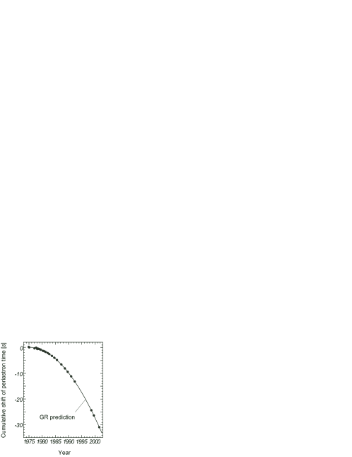
Figure 1: Cumulative shift of periastron time for the Hulse-Taylor pulsar according to observation (dots) and theory (solid line). The theoretical prediction takes into account the energy loss due to the emission of gravitational radiation.

Another very interesting system is J0737-3039, which in October 2003 was shown to consist of two pulsars with pulse periods of about $23$ milliseconds and $2.7$ seconds, respectively, and an orbital period of $2.4$ hours, and with an extremely high periastron advance of almost $17$ degrees per year. This is about four times larger than that of the Hulse-Taylor pulsar. Fortuitously, the system’s orbital orientation relative to our line of sight is almost exactly edge-on, which means that measurements of Shapiro time-delay of pulse periods of one component in the gravitational potential of the other can be performed with high precision. Presently the measurements of Shapiro delay verify GR predictions at the 0.1% level (Kramer et al. 2005). More results on this exciting system are expected in the near future.

The theory of black holes belongs to the most beautiful applications of GR. The structure of stationary black holes was completely clarified during a relatively short period of time. When matter disappears behind a horizon, an exterior observer sees almost nothing of its properties. One can no longer say, for example, how many baryons formed the black hole. A huge amount of information thus seems lost. The mass and angular momentum completely determine the external field, which is known analytically (Kerr solution). This led Wheeler to say that “a black hole has no hair” (Wheeler, 1971, p. 191-192). The preceding statement is now known as the no-hair-theorem.

The proof of this theorem is an outstanding contribution to mathematical physics, and was completed in the span of only a few years by various authors (Israel, Carter, Hawking, and Robinson). A decisive first step was taken by Israel (1967), who was able to show that a static black-hole solution of Einstein’s vacuum equation has to be spherically symmetric and, therefore, agree with the Schwarzschild solution. In a second paper Israel extended this result to black-hole solutions of the coupled Einstein-Maxwell system. The Reissner-Nordström $2$-parameter family, it turned out, exhausts the class of static so-called electrovac black holes. It was then conjectured by Israel, Penrose and Wheeler that in the stationary case the electrovac black holes should all be given by the $3$-parameter Kerr-Newman family. After a number of steps, supplied by various authors, this conjecture could finally be proven. See (Heusler, 1996) for a comprehensive account of black-hole uniqueness results.

The evidence for black holes in some X-ray binary systems and for super-massive black holes in galactic centers is still indirect, but has become overwhelming during the past few years. However, there is little evidence so far that these collapsed objects are described by the Kerr metric.

Until a few years ago the best one could say about the evidence for super-massive black holes in the center of some galaxies, was that it was compelling if dynamical studies and observations of active galactic nuclei were taken together. In the meantime the situation has improved radically. The beautiful work of Genzel and his coworkers has established a dark-mass concentration of about $3\times 10^{6}M_{\odot}$ near the center of the Milky Way with an extension of less than $17$ light hours (see, e.g., Ott et al., 2003). If this were a cluster of low mass stars or neutron stars, its central density would exceed $10^{17}M_{\odot}/pc^{3}$ and would not survive for more than a few $10^{5}$ years. The least exotic interpretation of this enormous dark mass concentration is that it is a black hole. But this is not the only possibility. Although alternative interpretations are highly implausible, they illustrate the point that dynamical studies alone cannot give an incontrovertible proof of the existence of black holes. Ideally, one would like to show that some black hole candidate actually has an event horizon. There have been various attempts in this direction, but presumably only gravitational wave astronomy will reveal the essential properties of black holes.

Most astrophysicists do not worry about possible remaining doubts. The evidence for (super-massive) black holes has become so overwhelming that the burden of proof is now on the hard-core skeptics.

6.6 Relativistic cosmology

In 1917 Einstein applied GR for the first time to cosmology, and found the first cosmological solution of a consistent theory of gravity (CPAE, Vol. 6, Doc. 43). In spite of its drawbacks this bold step can be regarded as the beginning of modern cosmology. It is still interesting to read this paper about which Einstein says: “I shall conduct the reader over the road that I have myself travelled, rather a rough and winding road, because otherwise I cannot hope that he will take much interest in the result at the end of the journey.” In a letter to Ehrenfest of February 4, 1917 (CPAE, Vol. 8, Doc. 294), Einstein wrote about his attempt: “I have again perpetrated something relating to the theory of gravitation that might endanger me of being committed to a madhouse.”

In his attempt Einstein assumed—and this was completely novel—that space is globally closed. This was because he believed at the time that this was the only way to satisfy what he later (CPAE, Vol. 7, Doc. 4) named Mach’s principle, the requirement that the metric field be determined uniquely by the energy-momentum tensor. In these early years, and for quite some time, Mach’s ideas on the origin of inertia played an important role in Einstein’s thinking (for a discussion, see, e.g., Janssen, 2005). This may even be the primary reason that he turned to cosmology so soon after the completion of GR. Einstein was convinced that isolated masses cannot impose a structure on space at infinity. His intention was to eliminate all vestiges of absolute space. It is for such reasons that he postulated a universe that is spatially finite and closed, a universe in which no boundary conditions are needed. Einstein was already thinking about the problem regarding the choice of boundary conditions at infinity in spring 1916. In a letter to Michele Besso from May 14, 1916 (CPAE, Vol. 8, Doc. 219) he mentions the possibility of the world being finite. A few month later he developed these ideas in correspondence with Willem de Sitter.

Einstein assumed that the Universe was not only closed but also static. This was not unreasonable at the time, because the relative velocities of the stars as observed were small.

These two assumptions, however, were incompatible with Einstein’s original field equations. For this reason, Einstein added the famous $\Lambda$-term, which is compatible with the principles of GR, in particular with the energy-momentum law $\nabla_{\nu}T^{\mu\nu}=0$ for matter. The modified field equations are (compare (77))

$$G_{\mu\nu}=(8\pi G/c^{4})T_{\mu\nu}-\Lambda g_{\mu\nu}\,.$$ (89)

The cosmological term is, in four dimensions, the only possible addition to the field equations if no higher than second order derivatives of the metric are allowed (Lovelock’s theorem; see Lovelock (1971)). This remarkable uniqueness is one of the most attractive features of general relativity. (In higher dimensions additional terms satisfying this requirement are allowed.)

For the static Einstein universe the field equations imply the two relations

$$(4\pi G/c^{2})\rho=\frac{1}{a^{2}}=\Lambda\,,$$ (90)

where $\rho$ is the mass density of the dust filled universe (zero pressure) and $a$ is the radius of curvature. (In passing we remark that the Einstein universe is the only static dust solution; one does not have to assume isotropy or homogeneity. Its instability was demonstrated by Lemaître in 1927.) Einstein was very pleased by this direct connection between the mass density and geometry, because he thought that this was in accord with Mach’s philosophy.

Einstein concludes with the following sentences:

“In order to arrive at this consistent view, we admittedly had to introduce an extension of the field equations of gravitation which is not justified by our actual knowledge of gravitation. It has to be emphasized, however, that a positive curvature of space is given by our results, even if the supplementary term is not introduced. That term is necessary only for the purpose of making possible a quasi-static distribution of matter, as required by the fact of the small velocities of the stars.” (CPAE, Vol. 6, Doc,  43, p. 551)

In a letter to De Sitter of March 12, 1917 (CPAE, Vol. 8, Doc. 311), Einstein emphasized that his model was intended primarily to settle the question “whether the basic idea of relativity can be followed through its completion, or whether it leads to contradictions”. He added that is was an entirely different matter whether the model corresponds to reality.

Only later did Einstein come to realize that Mach’s philosophy is predicated on an antiquated ontology that seeks to reduce the metric field to an epiphenomenon of matter. It became increasingly clear to him that the metric field has an independent existence (corresponding to physical degrees of freedom), and his enthusiasm for Mach’s principle gradually evaporated. In a letter to Pirani he wrote in 1954: “As a matter of fact, one should no longer speak of Mach’s principle at all.” (Pais, 1982, Sec. 15e). The absolute existence of the spacetime continuum, independent of any matter, is a remnant in GR of Newton’s absolute space and time. For a modern and comprehensive discussion of various aspects of Mach’s principle and their status in GR, see (Barbour & Pfister, 1995).

From static to expanding world models

It must have come as quite a shock to Einstein, that within days of receiving a letter in which Einstein described his cosmological model (CPAE, Vol. 8, Doc. 311), De Sitter had found a completely different cosmological model—also allowed by the new field equations with cosmological term—that was anti-Machian in that it contained no matter whatsoever (CPAE, Vol. 8, Doc. 312; De Sitter 1917a). For this reason, Einstein tried to discard it on various grounds (more on this below). Einstein and De Sitter mostly discussed De Sitter’s solution in its so-called static form (CPAE, Vol. 8, Doc. 355; De Sitter 1917b):

$$ds^{2}=-\Bigl{[}1-\left(\frac{r}{R}\right)^{2}\Bigr{]}c^{2}dt^{2}+\frac{dr^{2}}{1-(\frac{r}{R})^{2}}+r^{2}(d\vartheta^{2}+\sin^{2}\vartheta d\varphi^{2})\,.$$ (91)

The spatial metric is that of a three-sphere of radius $R$, determined by $\Lambda=3/R^{2}$. The model had one very interesting property: For light sources moving along static world lines there is a gravitational redshift, which became known as the De Sitter effect. This was thought to have some bearing on the redshift results obtained by Slipher. Because the fundamental (static) worldlines in this model are not geodesics, a freely- falling particle released by any static observer accelerates away from such an observer, generating local velocity (Doppler) redshifts corresponding to peculiar velocities. In his famous book, “The Mathematical Theory of Relativity”, Eddington wrote about this:

“De Sitter’s theory gives a double explanation for this motion of recession; first, there is the general tendency to scatter (…); second, there is a general displacement of spectral lines to the red in distant objects owing to the slowing down of atomic vibrations (…), which would be erroneously interpreted as a motion of recession.” (Eddington, 1924, p. 161)

We do not want to enter into all the confusion over the De Sitter universe (see, e.g., Vol. 8, pp. 351–357, the editorial note, “The Einstein-De Sitter-Weyl-Klein Debate”). One source of confusion was the apparent singularity at $r=R=(3/\Lambda)^{1/2}$. This was thoroughly misunderstood at first even by Einstein and Weyl. In the end, Einstein had to acknowledge that De Sitter’s solution is fully regular and matter-free and thus indeed a counterexample to Mach’s principle. But he still discarded the solution as physically irrelevant because it is not globally static. This is clearly expressed in a letter from Weyl to Klein, dated February 7, 1919 (quoted in CPAE, Vol. 8, Doc. 567, note 3), after Weyl had discussed the issue during a visit of Einstein to Zürich. An important discussion of the redshift of galaxies in De Sitter’s model by Weyl in 1923 should be mentioned. Weyl (1923) introduced an expanding version of the De Sitter model. For small distances his result reduced to what later became known as the Hubble law. Independently of Weyl, Lanczos (1922) also introduced a non-stationary interpretation of De Sitter’s solution in the form of a Friedmann spacetime with positive spatial curvature. In a subsequent paper he also derived the redshift for the non-stationary interpretation (Lanczos 1923).

Until about 1930 almost everybody ‘knew’ that the universe was static, notwithstanding two fundamental papers by Friedmann (1922, 1924) and independent work by Lemaître (1927). These path-breaking papers were largely ignored. The history of this early period has—as is often the case—been distorted by some widely read documents. Einstein too accepted the idea of an expanding universe only much later. After Friedmann’s first paper, he published a brief note claiming to have found an error in Friedmann’s work; when it was pointed out to him that it was his error, Einstein published a retraction of his comment, with a sentence that (fortunately for him) was deleted before publication: “[Friedmann’s paper] while mathematically correct is of no physical significance” (Stachel 2002, p. 469). In comments to Lemaître during the Solvay meeting in 1927, Einstein again rejected the expanding universe solutions as physically unacceptable. According to Lemaître, Einstein told him: “Vos calculs sont corrects, mais votre physique est abominable” (Schücking, 1993). On the other hand, we found in the archive of the ETH many years ago a postcard of Einstein to Weyl from 1923, related to Weyl’s reinterpretation of De Sitter’s solution, with the following interesting sentence: “If there is no quasi-static world, then away with the cosmological term.” This goes to show once again that history is not as simple as it is often being portrayed.

It is also not well-known that Hubble interpreted his famous results on the redshift of the radiation emitted by distant ‘nebulae’ in the framework of the De Sitter model. The general attitude is well illustrated by the following remark of Eddington at a Royal Society meeting in January 1930: “One puzzling question is why there should be only two solutions. I suppose the trouble is that people look for static solutions” (Eddington, 1930, p. 850). Lemaître, who had been for a short time a post-doctoral student of Eddington’s, read this remark in a report to the meeting published in Observatory, and wrote to Eddington alerting him to his 1927 paper. Eddington had seen that paper, but had completely forgotten about it. But now he was greatly impressed and praised Lemaître’s work in a letter to Nature. He also arranged for a translation which appeared in Monthly Notices of the Royal Astronomical Society (Lemaître 1931).

Lemaître’s successful explanation of Hubble’s discovery finally changed the viewpoint of the majority of workers in the field. At this point Einstein (1931) rejected the cosmological term as superfluous and no longer justified. At the end of the paper he made some remarks about the age problem which was quite severe without the $\Lambda$-term, since Hubble’s value for the Hubble parameter at the time was about seven times too large. Einstein, however, was not too worried and suggested two ways out. First, he pointed out that the matter distribution is in reality inhomogeneous and that the approximate treatment may be illusionary. Secondly, he cautioned against large extrapolations in time in astronomy.

Einstein repeated his new viewpoint much later (Einstein 1945), and it was adopted by many other influential workers, e.g., by Pauli (1958, supplementary note 19). Whether Einstein really considered the introduction of the $\Lambda$-term as “the biggest blunder of his life” as related by Gamov (1970, p. 44) appears doubtful to us. In his published work and extant letters such a strong statement is nowhere to be found. Einstein discarded the cosmological term merely for reasons of simplicity. For a minority of cosmologists this was not sufficient reason. Paraphrasing Rabi one could ask: ‘who ordered it away’?

Einstein’s paper (1931) was his last one on cosmology. In hindsight it is somewhat puzzling that after he saw the first paper by Friedmann he did not realize that his own static model was unstable.

Vacuum energy and gravity

So much for the classical discussion of the $\Lambda$-term; we do, however, want to add a few remarks the $\Lambda$-problem in the context of quantum theory, where the problem becomes very serious indeed. Since quantum physicists were facing so many other problems, it need not surprise us that in the early years they did not worry about this particular one. An exception was Pauli, who wondered in the early 1920s whether the zero-point energy of the radiation field could have significant gravitational effects. He estimated the influence of the zero-point energy of the electromagnetic radiation field—cut off at the classical electron radius—on the radius of the universe, and came to the conclusion that the “could not even reach to the moon” (for more on this, see Straumann 2003a). Pauli’s only published remark on his considerations can be found in his Handbuch article on quantum mechanics, in the section on the quantization of the radiation field, where he says: “Also, as is obvious from experience, the [zero-point energy] does not produce any gravitational field” (Pauli, 1933, p. 250).

For decades nobody else seems to have worried about contributions of quantum fluctuations to the cosmological constant, although physicists learned after Dirac’s hole theory that the vacuum state in quantum field theory is not empty but has interesting physical properties. As far as we know, the first one to come back to possible contributions of the vacuum energy density to the cosmological constant was Zel’dovich. He discussed this issue in two papers (Zel’dovich, 1967, 1968) during the third renaissance period of the $\Lambda$-term, but before the advent of spontaneously-broken gauge theories. He pointed out that, even if one assumes in a completely ad-hoc fashion that the zero-point contributions to the vacuum energy density are exactly cancelled by a bare term, there still remain higher-order effects. In particular, gravitational interactions between the particles in the vacuum fluctuations are expected on dimensional grounds to lead to a gravitational self-energy density of order $G\mu^{6}$, where $\mu$ is some cut-off scale. Even for $\mu$ as low as 1 GeV, this is about 9 orders of magnitude larger than the observational bound.

This strongly suggests that there is something profound that we do not seem to understand at all, certainly not in quantum field theory (nor, at least so far, in string theory). We are unable to calculate the vacuum energy density in quantum field theories, such as the Standard Model of particle physics. But we can attempt to make what appear to be reasonable order-of-magnitude estimates for the various contributions. All expectations are in dramatic conflict with the facts (see, e.g., Straumann, 2003b). Trying to arrange the cosmological constant to be zero is unnatural in a technical sense. It is like enforcing a particle to be massless, by fine-tuning the parameters of the theory when there is no symmetry principle implying a vanishing mass. The vacuum energy density is unprotected from large quantum corrections. This problem is particularly severe in field theories with spontaneous symmetry breaking. In such models there are usually several possible vacuum states with different energy densities. Furthermore, the energy density is determined by what is called the effective potential, and this is a dynamical object. Nobody can see any reason why the vacuum of the Standard Model we ended up as the universe cooled, has—by the standards of particle physics—an almost vanishing energy density. Most likely, we shall only find a satisfactory answer once we have a theory that successfully combines the concepts and laws of GR with those of quantum theory.

For a number of years now, cosmology has been going through a fruitful and exciting period. Some of the developments are clearly of general interest, well beyond the fields of astrophysics and cosmology. Lack of space prevents us from even indicating the most important issues of current interest.

Acknowledgements

We sincerely thank Thibault Damour for making valuable suggestions for improvements on an earlier draft version and Günther Rasche for carefully reading the manuscript.

References

- [1] Baade, W. and Zwicky, F. (1934a). On supernovae. Proceedings of the National Academy of Science (USA), 20, 254-259.
- [2] Baade, W. and Zwicky, F. (1934b). Cosmic rays from supernovae. Proceedings of the National Academy of Science (USA), 20, 259-263.
- [3] Barbour, J. and Pfister, H. (eds.) (1995). Mach’s principle: From Newton’s bucket to quantum gravity, Boston: Birkhäuser.
- [4] Bargmann, V. (1947). Irreducible unitary representations of the Lorentz group. Annals of Mathematics, 48, 568-640.
- [5] Bell, J.S. (1964). On the Einstein-Podolsky-Rosen paradox. Physics, 1, 195-200.
- [6] Bell, J.S. (1987). Speakable and unspeakable in quantum mechanics. Cambridge: Cambridge University Press.
- [7] Bertotti, B., Iess, L., and Tortora, P. (2003). A test of general relativity using radio links with the Cassini spacecraft. Nature, 425, 374-376.
-
[8]
Bohr, N. (1922).
The structure of the atom.
Nobel Lecture, December 11 1922.
http://nobelprize.org/physics/laureates/1922/bohr-lecture.html - [9] Bohr, N., H. A. Kramers, and J. C. Slater (1924). “The quantum theory of radiation” Philosophical Magazine 47: 785–802.
- [10] Bohr, N. and Rosenfeld, L. (1933). Zur Frage der Messbarkeit der elektromagnetischen Feldgrössen. Det Kongelige Danske Videnskabernes Selskab., Mathematisk-fysiske Meddelelser, Xii,8, 1-65.
- [11] Born, M. and Jordan, P. (1925). Zur Quantenmechanik. Zeitschrift für Physik, 34, 858-888.
- [12] Born, M. (2005). The Born-Einstein Letters 1916-1955. Basingstoke Hamphire (England): Macmillan.
- [13] Boulanger, N., Damour, T., Gualtieri, L, and Henneaux, M. (2001). Inconsistency of interacting, multi-graviton theories. Nuclear Physics B, 597, 127-171.
- [14] Breiman, L. (1968). Probability. Reading, Massachusetts: Addison-Wesley.
- [15] Chandrasekhar, S. (1934). Stellar configurations with degenerate cores. Observatory, 57, 373-77.
- [16] Christodoulou, D. and Klainerman, S. (1993). The global nonlinear stability of the Minkowski space. Princeton: Princeton University Press.
- [17] Chruściel, P.T. and Friedrich, H. (eds.) (2004). The Einstein equations and the large scale behaviour of gravitational fields. Basel: Birkhäuser.
- [18] Ciufolini, I. and Pavlis, E.C. (2004). A confirmation of the general relativistic prediction of the Lense-Thirring effect. Nature, 431, 958-960.
- [19] Clarke, C. (1994). A title of cosmic censorship. Classical and Quantum Gravity, 11, 1375-1386.
- [20] Coleman, S. and Mandula, J. (1967). All possible symmetries of the S matrix. Physical Review, 159, 1251-159.
- [21] Corvino, J. (2000). Scalar curvature deformation and a gluing construction for the Einstein constraint equations. Communications in Mathematical Physics, 214, 137-189.
- [22] CPAE, The collected papers of Albert Einstein, Edited by J. Stachel et al., Vols. 1-9. Princeton: Princeton University Press, 1987–2004.
- [23] Damour, T. and Schäfer, G. (1988). Higher-order relativistic periastron advances and binary pulsars. Il Nouvo Cimento, 101B, 127-176.
- [24] Damour, T. (2005). Poincaré, relativity, billiards and symmetry. arxiv.org/abs/hep-th/0501168.
- [25] Debye, P. (1910). Der Wahrscheinlichkeitsbegriff in der Theorie der Strahlung. Annalen der Physik (Leipzig), 33, 1427-1434.
- [26] Deser, S. (1970). Self-interaction and gauge invariance. General Relativity and Gravitation, 1, 9-18.
- [27] De Sitter, W. (1917a). “On the relativity of inertia. Remarks concerning Einstein’s latest hypothesis. ” Koninklijke Akademie van Wetenschappen te Amsterdam. Section of Sciences. Proceedings, 19, 1217-1225.
- [28] De Sitter, W. (1917b). “On the curvature of space.” Koninklijke Akademie van Wetenschappen te Amsterdam. Section of Sciences. Proceedings, 20, 229-243.
- [29] DeWitt-Morette, C. and DeWitt, B. (1988). Pin groups in physics. Physical Review D, 41, 1901-1907.
- [30] Dine, M. and Kusenko, A. (2004). The origin of the matter-antimatter asymmetry. Reviews of Modern Physics, 76, 1-30.
- [31] Dirac, P.A.M. (1931). Quantized singularities in the electromagnetic field. Proceedings of the Royal Society (London), A133, 357-400.
- [32] Earman, J. (1995). Bangs, crunches, whimpers, and shrieks. Singularities and acausalities in relativistic spacetimes. New York, Oxford: Oxford University Press.
- [33] Eddington, A.S. (1924). The mathematical theory of relativity, third (unaltered) edition (1975). New York: Chelsea Publishing Company.
- [34] Eddington, A.S. (1930). Space and its properties. Nature, 125, 849-850.
- [35] Ehlers, J. and Lämmerzahl, C. (eds.) (2006). Special Relativity: Will it survive the next 100 years ? Springer Lecture Notes in Physics. Berlin: Springer Verlag. to appear.
- [36] Ehlers, J. and Rindler, W. (1997). Local and global light bending in Einstein’s and other gravitational theories. General Relativity and Gravitation, 29, 519-529.
- [37] Ehrenfest, P. (1906). Zur Planck’schen Strahlungstheorie. Physikalische Zeitschrift, 7, 528-532.
- [38] Einstein, A. (1924). Quantentheorie des einatomigen idealen Gases. Sitzungsberichte der Preussischen Akademie der Wissenschaften (Gesamtsitzung) (Berlin), 261-267.
- [39] Einstein, A. (1925a). Quantentheorie des einatomigen idealen Gases. Zweite Abhandlung. Sitzungsberichte der Preussische Akademie der Wissenschaften (physikalisch-mathematische Klasse) (Berlin), 3-14.
- [40] Einstein, A. (1925b). Quantentheorie des idealen Gases. Sitzungsberichte der Preussische Akademie der Wissenschaften (physikalisch-mathematische Klasse) (Berlin), 18-25.
- [41] Einstein, A. (1931). Zum kosmologischen Problem der allgemeinen Relativitätstheorie. Sitzungsberichte der Preussischen Akademie der Wissenschaften (physikalisch-mathematische Klasse), 235-237.
- [42] Einstein, A. (1933). Einiges über die Entstehung der Allgemeinen Relativitätstheorie. Reprinted in Einstein (1977), p. 134-138.
- [43] Einstein, A., Podolsky, B., and Rosen, N. (1935). Can quantum-mechanical description of physical reality be considered complete? Physical Review, 47, 777-780.
- [44] Einstein, A. (1945). The meaning of relativity, appendix to the 2nd and following editions. Princeton Science Library. Princeton: Princeton University Press.
- [45] Einstein, A. (1952). Neun Aphorismen. In Essays presented to Leo Baeck on the occasion of his eightieth birthday. London: East & West Library.
- [46] Einstein, A. (1954). Notes on the origin of the general theory of relativity. In: Carl Seelig (ed.) Sonja Bargmann (trans.), Ideas and Opinions, p. 285-290. New York: Crown.
- [47] Einstein, A. (1977). Mein Weltbild. Carl Seeelig (ed.). Berlin: Ullstein Verlag. Translation: Ideas and Opinions. New York: Crown, 1954.
- [48] Einstein, A. (1979). Autobiographical notes. Translated and edited by P.A. Schilpp. La Salle (Illinois): Open Court.
- [49] Eisenstaedt, J. (1993). Lemaître and the Schwarzschild solution. In: J. Earman et al. (eds.), The attraction of gravitation. Boston: Birkhäuser. p. 353-389.
- [50] Euler, H. and Kockel, B. (1935). Über die Streuung von Licht an Licht nach der Dirac’schen Theorie. Naturwissenschaften, 23, 246-247.
- [51] Feynman R.P. (1985). QED – The Strange Theory of Light and Matter. Princeton: Princeton University Press.
- [52] Feynman, R.P. (1995). Lectures on gravitation. Reading, Massachusetts: Addison-Wesley.
- [53] Fierz, M. (1939). Über die relativistische Theorie kräftefreier Teilchen mit beliebigem Spin. Helvetica Physica Acta, 12, 3-37
- [54] Fierz, M. and Pauli, W. (1939). Relativistic wave equations for particles of arbitrary spin in an electromagnetic field. Proceedings of the Royal Society (London), A 173, 211-232.
- [55] Fock, V. (1926). Über die invariante Form der Wellen- und der Bewegungsgleichungen für einen geladenen Massenpunkt. Zeitschrift für Physik, 39, 226-232.
- [56] Fowler, R.H. (1926a). General forms of statistical mechanics with special reference to the requirements of the new quantum mechanics. Proceedings of the Royal Society (London), A 113, 432-449.
- [57] Fowler, R.H. (1926b). Dense matter. Monthly Notices of the Royal Astronomical Socienty (London), 87, 114-122.
- [58] Frauendiener, J., Giulini, D., and Perlick, V. (eds.) (2006). Mathematical Relativity: New Ideas and Developments, Springer Lecture Notes in Physics, Vol. 692. Berlin: Springer Verlag.
- [59] Friedmann, A. (1922). Über die Krümmung des Raumes. Zeitschrift für Physik 10, 377-386.
- [60] Friedmann, A. (1924). Über die Möglichkeit einer Welt mit konstanter negativer Krümmung des Raumes. Zeitschrift für Physik, 21, 326-332.
- [61] Friedrich, H. (1986). Existence and structure of past asymptotically simple solutions of Einstein’s field equations with positive cosmological constant. Journal of Geometry and Physics, 3, 101-117.
- [62] Frisch, R. (1933) Experimenteller Nachweis des Einsteinschen Strahlungsrückstoßes. Zeitschrift für Physik, 86, 42-48.
- [63] Fushchich, W. I., Shtelen, W. M., and Serov, N.I. (1993). Symmetry Analysis and Exact Solutions of Equations of Nonlinear Mathematical Physics. Dordrecht: Kluwer Academic Publishers.
- [64] Gamow, G. (1970). My World Line. New York: Viking Press.
- [65] Geroch, R. (1968). What is a singularity in GR? Annals of Physics (New York), 48, 526-540.
- [66] Giulini, D. (1997) Consistently implementing the field’s self-energy in Newtonian gravity. Physics Letters A, 232, 165-170.
- [67] Giulini, D. (2003). Close encounters of black holes. In: H. Falcke and F. Hehl (eds.), The galactic black hole – lectures on General Relativity and astrophysics. Bristol: Institute of Physics Publishing. Also: arxiv.org/abs/gr-qc/0302111.
- [68] Giulini, D. (2005a). Special Relativity—a first encounter. Oxford: Oxford University Press.
- [69] Giulini, D. (2005b). Algebraic and geometric aspects of Special Relativity. In: J. Ehlers and C. Lämmerzahl (eds.), Special Relativity: Will it survive the next 100 years. Springer Lecture Notes in Physics. Berlin: Springer Verlag (to appear).
- [70] Giulini, D. (2005c). Once more general covariance. Contribution to the FESt-workshop on Gravitation, Strings and Quantum Field Theory. Berlin: Springer Verlag (to appear).
- [71] Golfand, Y.A. and Likhtman, E.S. (1971). Extension of the algebra of the Poincaré group generators and violation of invariance. JETP Letters, 13, 323-326.
- [72] Gupta, S. (1954). Gravitation and electromagnetism. Physical Review, 96, 1683-1685.
- [73] Gupta, S. (1957). Einstein’s and other theories of gravitation. Reviews of Modern Physics, 29, 334-336
- [74] Hawking, S.W. and Ellis, G.F.R. (1973). The large scale structure of space-time. Cambridge: Cambridge University Press.
- [75] Heisenberg, W. and Pauli, W. (1929). Zur Quantenelektrodynamik der Wellenfelder. I. Zeitschrift für Physik, 56, 1- 61.
- [76] Heisenberg, W. and Pauli, W. (1930). Zur Quantenelektrodynamik der Wellenfelder. II. Zeitschrift für Physik, 59, 168- 190.
- [77] Heisenberg, W. and Euler, H. (1936). Folgerungen aus der Dirac’schen Theorie des Positrons. Zeitschrift für Physik, 98, 714-732.
- [78] Heusler, M. (1996). Black hole uniqueness theorems. Cambridge Lecture Notes in Physics, Vol. 6. Cambridge: Cambridge University Press.
- [79] Israel, W. (1967). Event horizons in static space-times. Physical Review, 164, 1776-1779.
- [80] Israel, W. (1987). Dark stars: the evolution of an idea. In: S.W. Hawking and W. Israel, Three hundred years of gravitation. Cambridge: Cambridge University Press (p. 215).
- [81] Jackson, J.D. and Okun, L.B. (2001). Historical roots of gauge invariance. Reviews of Modern Physics, 73, 663-680.
- [82] Janssen, M. (2005). Of pots and holes: Einstein’s bumpy road to general relativity. Annalen der Physik 14, Supplement: 58–85.
- [83] Jordan, P. and Pauli, W. (1928). Zur Quantenelektrodynamik ladungsfreier Felder. Zeitschrift für Physik, 47, 151-173.
- [84] Jost, R. (1957). Eine Bemerkung zum CTP Theorem. Helvetica Physica Acta, 30, 409-416.
- [85] Jost, R. (1965). The general theory of quantized fields. Providence, Rhode Island: American Mathematical Society.
- [86] Jost, R. (1995). Das Märchen vom Elfenbeinernen Turm, Reden und Aufsätze. K. Hepp, W. Hunziker, W. Kohn (eds.). Berlin: Springer Verlag.
- [87] Kaluza, T. (1921). Zum Unitätsproblem in der Physik. Sitzungsberichte der Preussischen Akademie der Wissenschaften zu Berlin (physikalisch-mathematische Klasse), 966-972.
- [88] Klein, O. (1926a). Quantentheorie und fünfdimensionale Relativitätstheorie. Zeitschrift für Physik, 37, 895-906.
- [89] Klein, O. (1926b). The Atomicity of electricity as a quantum law. Nature, 118, 516.
- [90] Klioner, S. and Soffel, M. (1998). Nonrotating astronomical relativistic reference frames. Astronomy and Astrophysics, 334, 1123-1135.
- [91] Kochen, S. and Specker, E. (1967). The problem of hidden variables in Quantum Mechanics. Journal of Mathematics and Mechanics, 17, 59-88.
- [92] Kogut. A., et al. (1993). Dipole anisotropy in the COBE differential microwave radiometers first-year sky maps. The Astrophysical Journal, 419, 1-6.
- [93] Kraichnan, R. (1955). Special relativistic derivation of generally covariant gravitation theory. Physical Review, 98, 1118-1122.
- [94] Kraichnan, R. (1956). Possibility of unequal gravitational and inertial mass. Physical Review, 101, 482-488.
- [95] Kramer, M., et al. (2005). Testing GR with the double pulsar: recent results. arxiv.org/abs/astro-ph/0503386.
- [96] Lanczos, K. (1922). Bemerkung zur de Sitterschen Welt. Physikalische Zeitschrift , 23, 539-543.
- [97] Lanczos, K. (1923). Über die Rotverschiebung in der de Sitterschen Welt. Zeitschrift für Physik, 17, 168-189.
- [98] Laue, M. (1911). Zur Dynamik der Relativitätstheorie. Annalen der Physik, 35, 524-542.
- [99] Lemaître, G.E. (1927). Un Univers homogène de masse constante et de rayon croissant, rendant compte de la vitesse radiale de nébuleuses extra-galactiques. Annales de la Société scientifique de Bruxelles, A47, 49.
- [100] Lemaître, G.E. (1931). A homogeneous universe of constant mass and increasing radius accounting for the radial velocity of extra-galactic nebulae. Monthly Notices of the Royal Astronomical Society (London), 91, 483-490.
- [101] Lewis, G. N. and Tolman, R. C. (1909). The principle of relativity, and non Newtonian mechanics. Philosophical Magazine 18: 510–523.
- [102] Lieb E. H. and Yau, H. T. (1987). The Chandrasekhar theory of stellar collapse as the limit of Quantum Mechanics. Communications in Mathematical Physics, 112, 147-174.
- [103] London, F. (1927). Quantenmechanische Deutung der Theorie von Weyl. Zeitschrift für Physik, 42, 375-389.
- [104] Lorentz, H. A. (1904). Electromagnetic phenomena in a system moving with any velocity smaller than that of light. Koninklijke Akademie van Wetenschappen te Amsterdam. Section of Sciences. Proceedings 6: 809–831.
- [105] Lovelock, D. (1971). The Einstein tensor and its generalizations. Journal of Mathematical Physics, 12, 498-501.
- [106] Lydon, T. J. and Sofia, S. (1996). A measurement of the shape of the solar disc: the solar quadrupole moment, the solar octopole moment, and the advance of perihelion of the planet Mercury. Physical Review Letters, 76, 177-179.
- [107] Lüders, G. and Zumino, B. (1958). Connection between spin and statsistics. Physical Review, 110, 1450-1453.
- [108] Mansouri, R. and Sexl, R. (1976). A test theory of Special Relativity I: simultaneity and clock synchronization. General Relativity and Gravitation, 8, 497-513.
- [109] Millikan, R.A. (1916). A direct photoelectric determination of Planck’s ‘’. Physical Review, 7, 355-388.
- [110] Mittelstaedt, P. (1970). Lorentzinvariante Gravitationstheorie. Köln and Opladen: Westdeutscher Verlag.
- [111] Müller, H., et al. (2003). Modern Michelson-Morley experiment using cryogenic optical resonators. Physical Review Letters, 91, 020401.
- [112] Nelson, E. (1967). Dynamic theory of Brownian motion. Princeton: Princeton University Press.
- [113] Newton, I. (1961). The correspondence of Isaac Newton, Vol. III, 1688-1694, H.W. Turnbull (ed.). Cambridge: Cambridge University Press.
- [114] Niederer, U.H. and O’Raifeartaigh, L. (1974). Realizations of the unitary representations of the inhomogeneous space-time groups I and II. Fortschritte der Physik, 22, 111-129 and 131-157.
- [115] Nordtvedt, K. (1988). Existence of the gravitomagnetic interaction. International Journal of Theoretical Physics, 27, 1395-1404.
- [116] Nordström, G. (1912). Relativitätsprinzip und Gravitation. Physikalische Zeitschrift 13: 1126–1129.
- [117] Nordström, G. (1913). Zur Theorie der Gravitation vom Standpunkt des Relativitätsprinzips. Annalen der Physik 42: 533–554.
- [118] Norton, J. (1992). Einstein, Nordström and the early demise of scalar, Lorentz-covariant theories of gravitation. Archive for the History of Exact Sciences, 45, 17-97.
- [119] Norton, J. (1993). Einstein and Nordström: some lesser-known thought experiments in gravitation. In: J. Earman et al. (eds.), The attraction of gravitation. Boston: Birkhäuser. p. 3-29.
- [120] Oppenheimer, J.R. (1930). On the theory of electrons and protons. Physical Review, 35, 562-563.
- [121] Oppenheimer, J.R. and Volkoff, G. (1939). On massive neutron cores. Physical Review, 55, 374-381.
- [122] Ott, T., et al. (2003). Inward bound: Studying the galactic center with NAOS/CONICA. ESO Messenger, 111, 1-8.
- [123] Pais, A. (1982). ‘Subtle is the Lord…’: The science and the life of Albert Einstein. Oxford: Oxford University Press.
- [124] Pais, A. (1991). Niels Bohr’s times in physics, philosophy, and polity. Oxford: Oxford University Press.
- [125] Pauli, W. (1933). Die allgemeinen Prinzipien der Wellenmechanik. Handbuch der Physik, Vol. XXIV (1933). New edition by N. Straumann (1990). Berlin: Springer-Verlag.
- [126] Pauli, W. (1940). The connection between spin and statistics. Physical Review, 56, 716-722.
- [127] Pauli, W. (1949). Einstein’s contributions to Quantum Theory. In: P. A. Schilpp (ed.), Albert Einstein: Philosopher-Scientist. Illinois: The Library of Living Philosophers.
- [128] Pauli, W. (1955). Exclusion principle, Lorentz group and reflexion of space-time and charge. In: W. Pauli (ed.), Niels Bohr and the Development of Physics. London: Pergamon Press.
- [129] Pauli, W. (1958). Theory of Relativity (Pergamon Press). Reprinted 1981. Mineola, New York: Dover Publications.
- [130] Pauli, W. (1985-99). Wissenschaftlicher Briefwechsel mit Bohr, Einstein, Heisenberg u.a. Vol. 1-4. K. von Meyenn (ed.). New York: Springer Verlag.
- [131] Pauli, W. (2000). Selected Topics in Field Quantization; Pauli Lectures on Physics, Vol. 6. Mineola, New York: Dover Publications.
- [132] Pireaux, S., Rozelot, J.-P., and Godier, S. (2003). Solar quadrupole moment and purely relativistic gravitation contributions to Mercury’s perihelion advance. Astrophysics and Space Science, 284, 1159-1194. Also: arxiv.org/abs/astro-ph/0109032.
- [133] Planck, M. (1911). Eine neue Strahlungshypothese. Verhandlungen der Deutschen Physikalischen Gesellschaft, 13, 138-148.
- [134] Poincaré, H. (1906). Sur la dynamique de l’électron. Rendiconti del Circulo Matematico di Palermo, 21, 129-146 and 166-175.
- [135] O’Raifeartaigh, L. and Straumann, N. (2000). Gauge theory: Historical origins and some modern developments. Reviews of Modern Physics, 72, 1-23.
- [136] Renn, J. (ed.) (Forthcoming). The genesis of General Relativity: Documents and interpretation. 4. Vols. New York: Springer.
- [137] Renn, J. and Schulmann, R. (1992). Albert Einstein–Mileva Maric. The love letters. Princeton: Princeton University Press.
- [138] Roepsdorff, G. (1996). Path integral approach to quantum physics. Berlin: Springer Verlag.
- [139] Roseveare, N. T. (1982). Mercury’s perihelion from Le Verrier to Einstein. Oxford: Clarendon Press.
- [140] Roxburgh, I.W. (2001). Gravitational multipole moments of the sun determined from helioseismic evidence of the internal structure and rotation. Astronomy and Astrophysics, 377, 688-690.
- [141] Saathoff, G., et al. (2003). Improved test of time dilation in Special Relativity. Physical Review Letters, 91, 190403.
- [142] Schrödinger, E. (1926). Über das Verhältnis der Heisenberg-Born-Jordan’schen Quantenmechanik zu der meinen. Annalen der Physik (Leipzig), 79, 734-756.
- [143] Schücking, E.L. (1993). Probleme der modernen Kosmologie in ihrer geschichtlichen Entfaltung. In Vom Urknall zum komplexen Universum. G. Börner, J. Ehlers, H. Meier (eds.). München: Piper.
- [144] Schweber, S.S. (1994). QED and the men who made it: Dyson, Feynman, Schwinger, and Tomonaga. Princeton: Princeton University Press.
- [145] Simon, B. (1979). Functional integration and quantum physics. Orlando: Academic Press.
- [146] Stachel, J. and Torretti, R. (1982). Einstein’s first derivation of mass-energy equivalence. American Journal of Physics, 50, 760-763.
- [147] Stachel, J. (2002). Einstein from B to Z. Boston: Birkhäuser.
- [148] Straumann, N. (1987). Zum Ursprung der Eichtheorien bei Hermann Weyl. Physikalische Blätter, 43, 414-421.
- [149] Straumann, N. (2002). Quantenmechanik. Berlin: Springer Verlag. Epilog, pp. 371.
- [150] Straumann, N. (2003a). The history of the cosmological constant problem. In On the nature of dark energy, IAP Astrophysics Colloquium 2002, Frontier Group, 2003, p. 17: Also: arxiv.org/abs/gr-qc/0208027.
- [151] Straumann, N. (2003b). On the cosmological constant problems and the astronomical evidence for a homogeneous energy density with negative pressure. In Poincaré Seminar 2002, vacuum energy – renormalization, 7-51. B. Duplantier, and V. Rivasseau (eds.). Boston: Birkhäuser. Also: arxiv.org/abs/astro-ph/0203330.
- [152] Straumann, N. (2005). On Einstein’s doctoral thesis. arxiv.org/abs/physics/0504201.
- [153] Streater, R.F. and Wightman, A.S. (1963). PCT, spin & and statistics, and all that (W.A. Benjamin, Inc., New York Amsterdam); reprinted 1989 in: Advanced Book Classics. Redwood City (CA): Addison Wesley.
- [154] Thirring, W. (1961). An alternative approach to the theory of gravitation. Annals of Physics (New York), 16, 96-117.
- [155] Thomas, L.H (1927). The calculations of atomic fields. Proceedings of the Cambridge Philosophical Socienty, 23, 542-548.
- [156] Thomas, L.T. (1927). The kinematics of an electron with an axis. Philosophical Magazine, 3, 1-22.
- [157] Uhlenbeck, G.E. and Ornstein, L.S. (1930). On the theory of Brownian motion. Physical Review, 36, 823-841.
- [158] Valiente-Kroon, J. (2003). Early radiative properties of the developments of time symmetric, conformally flat initial data. Classical and Quantum Gravity, 20, L53-L60.
- [159] Wald, R. (1986). Spin-two fields and general covariance. Physical Review D, 33, 3613-3625
- [160] Weinberg, S. (1964a). Derivation of gauge invariance and the equivalence principle from Lorentz invariance of the -matrix. Physics Letters, 9, 357-359.
- [161] Weinberg, S. (1964b). Photons and gravitons in -matrix theory: derivation of charge conservation and equality of gravitational and inertial mass. Physical Review, 135, B1049-B1056.
- [162] Weisskopf, V.S. (1936). Über die Elektrodynamik des Vakuums auf Grund der Quantentheorie des Elektrons. Det Kongelige Danske Videnskabernes Selskab, Matematisk-fysiske Meddelelser, 14, 1-39.
- [163] Wentzel, G. (1960). Quantum Theory of Fields (until 1947). In Theoretical physics in the twentieth century: A memorial volume to Wolfgang Pauli, M. Fierz and V.F. Weisskopf (eds.). New York: Interscience. pp. 48-77.
- [164] Weyl, H. (1918). Gravitation und Elektrizität. Sitzungsberichte der Königlich Preussischen Akademie der Wissenschaften zu Berlin (physikalisch-mathematische Klasse), 465-480. Also: Weyl (1968), Vol. II, Doc. 31, p. 29-42.
- [165] Weyl, H. (1919). Eine neue Erweiterung der Relativitätstheorie. Annalen der Physik 59: 101–133.
- [166] Weyl, H. (1923). Zur allgemeinen Relativitätstheorie. Physikalische Zeitschrift, 24, 230-232. Also: Weyl (1968), Vol. II, Doc. 56, p. 375-377.
- [167] Weyl, H. (1929). Elektron und Gravitation. I. Zeitschrift für Physik, 56, 330-352. Also: Weyl (1968), Vol. III, Doc. 85, p. 245-267.
-
[168]
Weyl, H. (1968).
Gesammelte Abhandlungen, Vol. I-IV.
K. Chandrasekharan (ed.). Berlin: Springer Verlag. - [169] Wheeler, J.A. (1971). From Mendeleev’s atom to the collapsing star. In: M. Verde (ed.) Atti del Convegno Mendeleeviano, p. 189-233. Torino: Accademia delle Science di Torino.
- [170] Wightman, A.S. (1972). The Dirac Equation. In Aspects of quantum theory. A. Salam, E.P. Wigner (eds.), 95-115. Cambridge: Cambridge University Press.
- [171] Wigner, E. (1929). Eine Bemerkung zu Einsteins neuer Formulierung des allgemeinen Relativitätsprinzips. Zeitschrift für Physik, 53, 592-596.
- [172] Wigner, E. (1939). On unitary representations of the inhomogeneous Lorentz group Annals of Mathematics, 40, 149-204.
- [173] Wigner, E. (1993). Collected Works. A. Wightman (ed.). Berlin: Springer Verlag.
- [174] Will, C. (1993). Theory and experiment in gravitational physics, 2nd revised edition. Cambridge: Cambridge University Press.
- [175] Wolf, P., et al. (2003). Test of Lorentz invariance using a microwave resonator. Physical Review Letters, 90, 060402.
- [176] Wyss, W. (1965). Zur Unizität der Gravitationstheorie. Helvetica Physica Acta, 38, 469-480.
- [177] Zeldovich, Ya.B. (1967). Cosmological constant and elementary particles. Journal of Experimental and Theoretical Physics. Letters, 61, 316-317.
- [178] Zeldovich, Ya.B. (1968). The cosmological constant and the theory of elementary particles. Soviet Physics Uspekhi, 11, 381-393.
- [179] Zhang, D.Z. (1993). C.N. Yang and contemporary mathematics. The Mathematical Intelligencer, 15 No. 4 (Fall), 13-21.