Lancret helices

Abstract

Helical configurations of inhomogeneous symmetric rods with non-constant bending and twisting stiffness are studied within the framework of the Kirchhoff rod model. From the static Kirchhoff equations, we obtain a set of differential equations for the curvature and torsion of the centerline of the rod and the Lancret’s theorem is used to find helical solutions. We obtain a free standing helical solution for an inhomogeneous rod whose curvature and torsion depend on the form of variation of the bending coefficient along the rod. These results are obtained for inhomogeneous rods without intrinsic curvature, and for a particular case of intrinsic curvature.

1 Introduction

Helical filaments are tridimensional structures commonly found in Nature. They can be seen in microscopic systems, as biomolecules [1], bacterial fibers [2] and nanosprings [3], and in macroscopic ones, as ropes, strings and climbing plants [4, 5, 6]. Usually, the axis of all these objects is modeled as a circular helix, i. e. a 3D-space curve whose mathematical geometric properties, namely the curvature, $k_{F}$, and the torsion, $\tau_{F}$, are constant [7, 8, 9]. This kind of helical structure has been shown to be a static solution of the Kirchhoff rod model [7].

The Kirchhoff rod model [10, 11] has been proved to be a good framework to study the statics [7, 12, 13] and dynamics [29] of long, thin and inextensible elastic rods. Applications of the Kirchhoff model range from Biology [1, 14, 5] to Engineering [15] and, recently, to Nanoscience [16]. In most cases, the rod or filament is considered as being homogeneous, but the case of nonhomogeneous rods have also been considered in the literature. It has been shown that nonhomogeneous Kirchhoff rods may present spatial chaos [17, 18]. In the case of planar rods, Domokos and collaborators have provided some rigorous results for non-uniform elasticae [19] and for constrained Euler buckling [20, 21]. Deviations of the helical structure of rods due to periodic variation of the Young’s modulus were verified numerically by da Fonseca, Malta and de Aguiar [22]. Nonhomogeneous rods subject to given boundary conditions were studied by da Fonseca and de Aguiar in [23]. The effects of a nonhomogeneous mass distribution in the dynamics of unstable closed rods have been analyzed by Fonseca and de Aguiar [24]. Goriely and McMillen [25] studied the dynamics of cracking whips [26] and Kashimoto and Shiraishi [27] studied twisting waves in inhomogeneous rods.

The stability analysis of helical structures is of great importance in the study of the elastic behavior of filamentary systems and has been performed both experimentally [28] and theoretically [29, 30, 31]. It has been also shown that the type of instability in twisted rods strongly depends on the anisotropy of the cross section [32, 33, 34].

Here, we consider a rod with nonhomogeneous bending and twisting coefficients varying along its arclength $s$, $B(s)$ and $C(s)$, respectively. We are concerned with the following question: is there any helical solution for the stationary Kirchhoff equations in the case of an inhomogeneous rod ? The answer is ‘yes’ and it will be shown that the helical solution for an inhomogeneous rod with varying bending coefficient cannot be the well known circular helix, for which the curvature, $k_{F}$, and torsion, $\tau_{F}$, are constant. To this purpose, we shall derive a set of differential equations for the curvature and the torsion of the centerline of an inhomogeneous rod and then apply the condition that a space curve must satisfy to be helical: the Lancret’s theorem. We shall obtain the simplest helical solutions satisfying the Lancret’s theorem and show that they are free standing helices, i.e., helices that are not subjected to axial forces [30]. A resulting helical structure different from the circular helix, from now on, will be called a Lancret helix.

According to the fundamental theorem for space curves [9], the curvature $k_{F}(s)$, and the torsion, $\tau_{F}(s)$, completely determine a space curve, but for its position in space. We shall show that the $k_{F}(s)$ and $\tau_{F}(s)$ of a Lancret helix depend directly on the bending coefficient, $B(s)$, an expected result since the centerline of the rod does not depend on the twisting coefficient (see for example, Neukirch and Henderson [13]).

Some motivations for this work are related to defects [35] and distortions [36] in biological molecules. These defects and distortions could be modeled as inhomogeneities along a continuous elastic rod.

In Sec. II we review the general definition of a space curve, the Frenet basis and the so-called Lancret’s theorem. In Sec. III we present the static Kirchhoff equations for an intrinsically straight rod with varying stiffness, and derive the differential equations for the curvature and torsion of the rod. In Sec. IV we use the Lancret’s theorem for obtaining helical solutions of the static Kirchhoff equations and we show that they cannot be circular helices if the bending coefficient is not constant. As illustration, we compare a homogeneous rod with two simple cases of inhomogeneous rods: (i) linear and (ii) periodic bending coefficient varying along the rod. The circular helix has a well known relation of the curvature and torsion with the radius and pitch of the helix. In Sec. V we define a function involving all these variables in such a way that for the circular helix its value is identically null. We have verified, numerically, that this function approaches zero for the inhomogeneous cases considered here. In Sec. VI we analyse the cases of null torsion (straight and planar rods). Since helical solutions of intrinsically straight rods are not dynamically stable [30], in Sec. VII we consider a rod with a given helical intrinsic curvature and we obtain, for this case, a helical solution of the static Kirchhoff equations similar to that of an intrinsically straight inhomogeneous rod. In Sec. VIII we summarize the main results.

2 Curves in space

A curve in space can be considered as a path of a particle in motion. The rectangular coordinates $(x,y,z)$ of the point on a curve can be expressed as function of a parameter $u$ inside a given interval:

$$x=x(u)\;,\;\;y=y(u)\;,\;\;z=z(u)\;,\;\;\;u_{1}\leq u\leq u_{2}\;.$$ (1)

We define the vector ${\mathbf{x}}(u)\equiv(x(u),y(u),z(u))$. If $u$ is the time, ${\mathbf{x}}(u)$ represents the trajectory of a particle.

2.1 The Frenet frame and the Frenet-Serret equations

The vector tangent to the space curve at a given point $P$ is simply $d{\mathbf{x}}/du$. It is possible to show [9] that if the arclength $s$ of the space curve is considered as its parameter, the tangent vector at a given point $P$ of the curve ${\mathbf{x}}(s)$ is a unitary vector. So, using the arclength $s$ to parametrize the curve, we shall denote by ${\mathbf{t}}$ its tangent vector

$${\mathbf{t}}=\frac{d{\mathbf{x}}}{ds}\;,$$ (2)

$\|{\mathbf{t}}\|=1$. The tangent vector ${\mathbf{t}}$ points in the direction of increasing $s$.

The plane defined by the points $P_{1}$, $P_{2}$ and $P_{3}$ on the curve, with $P_{2}$ and $P_{3}$ approaching $P_{1}$, is called the osculating plane of the curve at $P_{1}$ [9]. Given a point $P$ on the curve, the principal normal at $P$ is the line, in the osculating plane at $P$, that is perpendicular to the tangent vector at $P$. The normal vector ${\mathbf{n}}$ is the unit vector associated to the principal normal (its sense may be chosen arbitrarily, provided it is continuous along the space curve).

From ${\mathbf{t}}.{\mathbf{t}}=1$, differentiating with respect to $s$ (indicated by a prime) it follows that:

$${\mathbf{t}}.{\mathbf{t}}^{\prime}=0\;,$$ (3)

so that ${\mathbf{t}}$ and ${\mathbf{t}}^{\prime}$ are orthogonal. It is possible to show that ${\mathbf{t}}^{\prime}$ lies in the osculating plane, consequently ${\mathbf{t}}^{\prime}$ is in the direction of ${\mathbf{n}}$. This allows us to write

$${\mathbf{t}}^{\prime}=k_{F}\,{\mathbf{n}}\;,$$ (4)

$k_{F}$ being called the curvature of the space curve at $P$.

The curvature measures the rate of change of the tangent vector when moving along the curve. In order to measure the rate of change of the osculating plane, we introduce the vector normal to this plane at $P$: the binormal unit vector ${\mathbf{b}}$. At a point $P$ on the curve, ${\mathbf{b}}$ is defined in such a way that

$${\mathbf{b}}={\mathbf{t}}\times{\mathbf{n}}\;.$$ (5)

The frame $\{{\mathbf{n}},{\mathbf{b}},{\mathbf{t}}\}$ can be taken as a new frame of reference and forms the moving trihedron of the curve. It is commonly called the Frenet frame. The rate of change of the osculating plane is expressed by the vector ${\mathbf{b}}^{\prime}$. It is possible to show that ${\mathbf{b}}^{\prime}$ is anti-parallel to the unit vector ${\mathbf{n}}$ [9]. So we can write

$${\mathbf{b}}^{\prime}=-\tau_{F}\,{\mathbf{n}}\;,$$ (6)

$\tau_{F}$ being called the torsion of the space curve at $P$.

The rate of variation of ${\mathbf{n}}$ [9] can be obtained straightforwardly. It is given by

$${\mathbf{n}}^{\prime}=-k_{F}\,{\mathbf{t}}+\tau_{F}\,{\mathbf{b}}\;.$$ (7)

The set of differential equations for $\{{\mathbf{t}},{\mathbf{n}},{\mathbf{b}}\}$ is

$$\begin{array}[]{l}{\mathbf{t}}^{\prime}=k_{F}\,{\mathbf{n}}\;,\\ {\mathbf{n}}^{\prime}=-k_{F}\,{\mathbf{t}}+\tau_{F}\,{\mathbf{b}}\;,\\ {\mathbf{b}}^{\prime}=-\tau_{F}\,{\mathbf{n}}\;,\end{array}$$ (8)

and are known as the formulas of Frenet or the Serret-Frenet equations [9].

2.2 The Fundamental theorem of space curves

A space curve parametrized by its arclength $s$ is defined by a vectorial function ${\mathbf{x}}(s)$. The form of ${\mathbf{x}}(s)$ depends on the choice of the coordinate system. Nevertheless, there exists a form of characterization of a space curve given by a relation that is independent of the coordinates. This relation gives the natural equation for the curve.

$k_{F}(s)$ gives the natural equation in the case of planar curves. Indeed, if $\varphi$ is the angle between the tangent vector of the planar curve and the $x$-axis of the coordinate system, it is possible to show that $k_{F}=d\varphi/ds$. Since $\cos(\varphi)=dx/ds$ and $\sin(\varphi)=dy/ds$, knowing $k_{F}(s)$, then $\varphi(s)$, $x(s)$, and $y(s)$ of the planar curve can be obtained immediatly:

$$\varphi(s)=\int_{s_{0}}^{s}k_{F}(s)\,ds,\;\;x(s)=\int_{s_{0}}^{s}\cos\varphi(s)ds,\;\;y(s)=\int_{s_{0}}^{s}\sin\varphi(s)ds.$$ (9)

In the case of non-planar curves, if we have two single valued continuous functions $k_{F}(s)$ and $\tau_{F}(s),\;s>0,$ then there exists one and only one space curve, determined but for its position in space, for which $s$ is the arclength, $k_{F}(s)$ the curvature, and $\tau_{F}(s)$ the torsion. It is the Fundamental theorem for space curves [9]. The functions $k_{F}(s)$ and $\tau_{F}(s)$ provide the natural equations of the space curve.

2.3 Curves of constant slope: the Lancret’s theorem

A space curve ${\mathbf{x}}(s)$ is a helix if the lines tangent to ${\mathbf{x}}$ make a constant angle with a fixed direction in space (the helical axis) [8, 9]. Denoting by ${\mathbf{a}}$ the unit vector of this direction, a helix satisfies

$${\mathbf{t}}.{\mathbf{a}}=\cos\alpha=\mbox{constant}\;.$$ (10)

Differentiating Eq. (10) with respect to $s$ gives ${\mathbf{a}}.{\mathbf{n}}=0$. Therefore ${\mathbf{a}}$ lies in the plane determined by the vectors ${\mathbf{t}}$ and ${\mathbf{b}}$:

$${\mathbf{a}}={\mathbf{t}}\cos\alpha+{\mathbf{b}}\sin\alpha\;.$$ (11)

Differentiating Eq. (11) with respect to $s$, gives

$$0=(k_{F}\,\cos\alpha-\tau_{F}\,\sin\alpha){\mathbf{n}}\;,$$

or

$$\frac{k_{F}}{\tau_{F}}=\tan\alpha=\mbox{constant.}$$ (12)

This result says that for curves of constant slope the ratio of curvature over torsion is constant. Conversely, given a regular curve for which the equation (12) is satisfied, it is possible to find [9] a constant angle $\alpha$ such that

$${\mathbf{n}}\left(k_{F}\cos\alpha-\tau_{F}\sin\alpha\right)=0\;,$$

$$\frac{d}{ds}\left({\mathbf{t}}\cos\alpha+{\mathbf{b}}\sin\alpha\right)=0\;,$$

implying that the vector $\mathbf{a}={\mathbf{t}}\cos\alpha+{\mathbf{b}}\sin\alpha$ is the unit vector along the axis. Moreover, ${\mathbf{a}}.{\mathbf{t}}=\cos\alpha$=constant, so that the curve has constant slope. This result can be expressed as:

A necessary and suficient condition for a space curve to be a curve of constant slope (a helix) is that the ratio of curvature over torsion be constant. It is the well known Lancret’s theorem, dated of 1802 and first proved by B. de Saint Venant [9, 37].

If a helical curve ${\mathbf{x}}(s)$ is projected onto the plane perpendicular to ${\mathbf{a}}$, the vector ${\mathbf{x}}_{1}(s)$ representing this projection is given by

$${\mathbf{x}}_{1}(s)={\mathbf{x}}-({\mathbf{x}}.{\mathbf{a}}){\mathbf{a}}\;.$$ (13)

It is possible to show [9] that the curvature $k_{1}$ of the projected curve is given by:

$$k_{1}(s)=\frac{k_{F}(s)}{\sin^{2}\alpha}\;.$$ (14)

The shape of the planar curve obtained by projecting a helical curve onto the plane perpendicular to its axis is used to characterize it. For example, the well known circular helix projects a circle onto the plane perpendicular to its axis. The spherical helix projects an arc of an epicycloid onto a plane perpendicular to its axis [9]. The logarithmic spiral is the projection of a helical curve called conical helix [9].

3 The static Kirchhoff equations

The statics and dynamics of long and thin elastic rods are governed by the Kirchhoff rod model. In this model, the rod is divided in segments of infinitesimal thickness to which the Newton’s second law for the linear and angular momentum are applied. We derive a set of partial differential equations for the averaged forces and torques on each cross section and for a triad of vectors describing the shape of the rod. The set of PDE are completed with a linear constitutive relation between torque and twist.

The central axis of the rod, hereafter called centerline, is represented by a space curve ${\mathbf{x}}$ parametrized by the arclength $s$. A Frenet frame is defined for this space curve as described in the previous section. For a physical filament the use of a local basis, $\{{\mathbf{d}}_{1},{\mathbf{d}}_{2},{\mathbf{d}}_{3}\}$, to describe the rod has the advantage of taking into account the twist deformation of the filament. This local basis is defined such that ${\mathbf{d}}_{3}$ is the vector tangent to the centerline of the rod (${\mathbf{d}}_{3}={\mathbf{t}}$), and ${\mathbf{d}}_{1}$ and ${\mathbf{d}}_{2}$ lie on the cross section plane. The local basis is related to the Frenet frame $\{{\mathbf{n}},{\mathbf{b}},{\mathbf{t}}\}$ through

$$({\mathbf{d}}_{1}\;{\mathbf{d}}_{2}\;{\mathbf{d}}_{3})=({\mathbf{n}}\;{\mathbf{b}}\;{\mathbf{t}})\left(\begin{array}[]{ccc}\cos\xi&-\sin\xi&0\\ \sin\xi&\cos\xi&0\\ 0&0&1\end{array}\right)\;,$$ (15)

where the angle $\xi$ is the amount of twisting of the local basis with respect to ${\mathbf{t}}$.

In this paper, we are concerned with equilibrium solutions of the Kirchhoff model, so our study departs from the static Kirchhoff equations [38]. In scaled variables, for intrinsically straight isotropic rods, these equations are:

$$\mathbf{F}^{\prime}=0\;,$$ (16)

$$\mathbf{M}^{\prime}=\mathbf{F}\times\mathbf{d}_{3}\;,$$ (17)

$$\mathbf{M}=B(s)\,k_{1}\,\mathbf{d}_{1}+B(s)\,k_{2}\,\mathbf{d}_{2}+C(s)\,k_{3}\,\mathbf{d}_{3}\;,$$ (18)

the vectors $\mathbf{F}$ and $\mathbf{M}$ being the resultant force, and corresponding moment with respect to the centerline of the rod, respectively, at a given cross section. As in the previous section, $s$ is the arclength of the rod and the prime ^′ denotes differentiation with respect to $s$. $k_{i}$ are the components of the twist vector, $\mathbf{k}$, that controls the variations of the director basis along the rod through the relation

$${\mathbf{d}}^{\prime}_{i}={\mathbf{k}}\times{\mathbf{d}}_{i}\;,\;\;i=1,2,3\;.$$ (19)

$k_{1}$ and $k_{2}$ are related to the curvature of the centerline of the rod $(k_{F}=\sqrt{k^{2}_{1}+k^{2}_{2}})$ and $k_{3}$ is the twist density. $B(s)$ and $C(s)$ are the bending and twisting coefficients of the rod, respectively. In the case of macroscopic filaments the bending and twisting coefficients can be related to the cross section radius and the Young’s and shear moduli of the rod. Writing the force $\mathbf{F}$ in the director basis,

$${\bf{F}}=f_{1}{\bf{d}}_{1}+f_{2}{\bf{d}}_{2}+f_{3}{\bf{d}}_{3}\;,$$ (20)

the equations (16–18) give the following differential equations for the components of the force and twist vector:

$$f^{\prime}_{1}-f_{2}\,k_{3}+f_{3}\,k_{2}=0\;,$$ (21)

$$f^{\prime}_{2}+f_{1}\,k_{3}-f_{3}\,k_{1}=0\;,$$ (22)

$$f^{\prime}_{3}-f_{1}\,k_{2}+f_{2}\,k_{1}=0\;,$$ (23)

$$(B(s)\,k_{1})^{\prime}+(C(s)-B(s))\,k_{2}\,k_{3}-f_{2}=0\;,$$ (24)

$$(B(s)\,k_{2})^{\prime}-(C(s)-B(s))\,k_{1}\,k_{3}+f_{1}=0\;,$$ (25)

$$(C(s)\ k_{3})^{\prime}=0\;.$$ (26)

The equation (26) shows that the component $M_{3}=C(s)\,k_{3}$ of the moment in the director basis (also called torsional moment), is constant along the rod, consequently the twist density $k_{3}$ is inversely proportional to the twisting coefficient $C(s)$

$$k_{3}(s)=\frac{M_{3}}{C(s)}\;.$$ (27)

In order to look for helical solutions of the Eqs. (21–26) the components of the twist vector $\mathbf{k}$ are expressed as follows:

$$k_{1} = k_{F}(s)\sin\xi\;,$$ (28)

$$k_{2} = k_{F}(s)\cos\xi\;,$$ (29)

$$k_{3} = \xi^{\prime}+\tau_{F}(s)\;,$$ (30)

where $k_{F}(s)$ and $\tau_{F}(s)$ are the curvature and torsion, respectively, of the space curve that defines the centerline of the rod and $\xi$ is given by Eq. (15). If the rod is homogeneous, the helical solution has constant $k_{F}$ and $\tau_{F}$, and $\xi^{\prime}$ is proved to be null [5].

Substituting Eqs. (28–30) in Eqs. (21–26), extracting $f_{1}$ and $f_{2}$ from Eqs. (25) and (24), respectively, differentiating them with respect to $s$, and substituting in Eqs. (21), (22) and (23), gives the following set of nonlinear differential equations:

$$[M_{3}\,k_{F}(s)-B(s)\,k_{F}(s)\,\tau_{F}(s)]^{\prime}-(B(s)\,k_{F}(s))^{\prime}\,\tau_{F}(s)=0\;,$$ (31)

$$(B(s)\,k_{F}(s))^{\prime\prime}+k_{F}(s)\,\tau_{F}(s)[M_{3}-B(s)\,\tau_{F}(s)]-f_{3}(s)\,k_{F}(s)=0\;,$$ (32)

$$(B(s)\,k_{F}(s))^{\prime}\,k_{F}(s)+f^{\prime}_{3}(s)=0\;.$$ (33)

Appendix A presents the details of the derivation of Eqs. (31–33).

The Eqs. (31–33) for the curvature, $k_{F}$, and torsion, $\tau_{F}$ do not depend on the twisting coefficient, $C(s)$. Therefore, the centerline of an inhomogeneous rod does not depend on the twisting coefficient like in the case of homogeneous rods (see, for example, Eqs. (13) and (14) of Ref. [13]).

Langer and Singer [39] have obtained a set of first-order ordinary differential equations for the curvature and torsion of the centerline of a homogeneous rod that contains terms proportional to $k_{F}^{2}$ and $\tau^{2}_{F}$. The Eqs. (31–33) have the advantage of involving only terms linear in $k_{F}$ and $\tau_{F}$.

4 Helical solutions of inhomogeneous rods

In order to find helical solutions for the static Kirchhoff equations, we apply the Lancret’s theorem to the general equations (31–33). We first rewrite the Lancret’s theorem in the form:

$$k_{F}(s)=\beta\,\tau_{F}(s)\;,$$ (34)

with $\beta\neq 0$. From Eq. (12),

$$\beta\equiv\tan\alpha=\mbox{Constant}\;.$$ (35)

Substituting Eq. (34) in Eq. (31) we obtain

$$\tau_{F}^{\prime}\,(M_{3}-B\,\tau_{F})-2\,\tau_{F}\,(B\,\tau_{F})^{\prime}=0\;.$$ (36)

Substituting Eq. (34) in Eq. (32) and extracting $f_{3}$, we obtain

$$f_{3}=\frac{(B\,\tau_{F})^{\prime\prime}}{\tau_{F}}+\tau_{F}\,(M_{3}-B\,\tau_{F})\;.$$ (37)

Differentiating $f_{3}$ with respect to $s$ and substituting in Eq. (33) we obtain the following differential equation for $\tau_{F}$:

$$\frac{(B\,\tau_{F})^{\prime\prime\prime}}{\tau_{F}}-\frac{(B\,\tau_{F})^{\prime\prime}\tau_{F}^{\prime}}{\tau_{F}^{2}}+(\beta^{2}+1)\,\tau_{F}\,(B\,\tau_{F})^{\prime}=0\;,$$ (38)

where the Eq. (36) was used to simplify the above equation. One immediate solution for this differential equation is

$$(B\,\tau_{F})^{\prime}=0\;,$$ (39)

that substituted in Eq. (36) gives

$$\tau_{F}^{\prime}\,(M_{3}-B\tau_{F})=0\;.$$ (40)

For non-constant $\tau_{F}$, the Eq. (40) gives the following solution for $\tau_{F}$:

$$\tau_{F}(s)=\frac{M_{3}}{B(s)}\;.$$ (41)

Substituting the Eqs. (39) and (41) in Eq. (37) we obtain that

$$f_{3}(s)=0\;.$$ (42)

Substituting Eq. (41) in (34) we obtain:

$$k_{F}(s)=\beta\frac{M_{3}}{B(s)}\;.$$ (43)

Substituting Eq. (15) in Eq. (20), the force ${\bf{F}}$ becomes

$${\bf{F}}=(f_{1}\cos\xi-f_{2}\sin\xi)\,{\bf{n}}+(f_{1}\sin\xi+f_{2}\cos\xi)\,{\bf{b}}+f_{3}\,{\bf{t}}\;,$$ (44)

where $\{{\bf{n}},{\bf{b}},{\bf{t}}\}$ is the Frenet basis. Using the Eqs. (88) and (89) for $f_{1}$ and $f_{2}$ (Appendix A), we obtain

$${\bf{F}}=-(B\,k_{F})^{\prime}\,{\bf{n}}+k_{F}\,[M_{3}-B\,\tau_{F}]\,{\bf{b}}+f_{3}\,{\bf{t}}\;,$$ (45)

where $f_{3}$, in the inhomogeneous case, must satisfy the Eq. (33).

Substituting the Eqs. (41–43) in the Eq. (45), and using Eq. (35), it follows ${\bf{F}}=0$. Therefore, the helical solutions satisfying (39) are free standing.

Now, we prove that a circular helix cannot be a solution of the static Kirchhoff equations for a rod with varying bending stiffness. If a helix is circular, $k_{F}^{\prime}=0$ and $\tau_{F}^{\prime}=0$, and from Eq. (31) we obtain:

$$2\,k_{F}\,\tau_{F}\,B^{\prime}=0\;.$$ (46)

Since $B^{\prime}(s)\neq 0$, Eq. (46) will be satisfied only if $k_{F}=0$ and/or $\tau_{F}=0$. Therefore, it is not possible to have a circular helix as a solution for a rod with varying bending coefficient.

The solutions for the curvature $k_{F}$, Eq. (43), and the torsion $\tau_{F}$, Eq. (41), can be used to obtain the unit vectors of the Frenet frame (by integration of the Eqs. (8)). From Eqs. (43), (35) and (11), we can obtain $\alpha$ and ${\bf{a}}$ once $k_{F}(0)$, $M_{3}$ and $B(s)$ are given. By choosing the $z$-direction of the fixed cartesian basis as the direction of the unit vector ${\mathbf{a}}$, we can integrate ${\mathbf{t}}$ in order to obtain the three-dimensional configuration of the centerline of the rod.

Figure 1 displays the helical solution of the static Kirchhoff equations for rods with bending coefficients given by

$$\mbox{Fig \ref{fig1}a:}\;\;\;B_{a}(s) = 1\;,$$ (47)

$$\mbox{Fig \ref{fig1}b:}\;\;\;B_{b}(s) = 1+0.007\,s\;\;,$$ (48)

$$\mbox{Fig \ref{fig1}c:}\;\;\;B_{c}(s) = 1+0.1\,\sin(0.04s+2)\;\;.$$ (49)

The case of constant bending (47) produces the well known circular helix displayed in Fig. 1a. Figs. 1b–1c show that non-constant bending coefficients (Eqs. (48–49)) do not produce a circular helix.

The helical solutions displayed in Fig. 1 satisfy the Lancret’s theorem, Eq. (12). The tridimensional helical configurations displayed in Fig. 1 were obtained by integrating the Frenet-Serret equations (8) using the following initial conditions for the Frenet frame: ${\mathbf{t}}(s=0)=(0,\sin\alpha,\cos\alpha)$, ${\mathbf{n}}(s=0)=$ $(-1,0,0)$ and ${\mathbf{b}}(s=0)=$ $(0,-\cos\alpha,\sin\alpha)$. This choice ensures that the $z$-axis is parallel to the direction of the helical axis, vector ${\mathbf{a}}$. The centerline of the helical rod is a space curve ${\mathbf{x}}(s)=(x(s),y(s),z(s))$ that is obtained by integration of the tangent vector ${\mathbf{t}}(s)$. We have taken the helical axis as the $z$-axis and placed the initial position of the rod at $x(0)=1/k_{1}(0)$, $y(0)=0$ and $z(0)=0$ (in scaled units), where $k_{1}(0)$ is the curvature of the planar curve at $s=0$ obtained by projecting the space curve onto the plane perpendicular to the helical axis (Eq. (14)). From Eq. (14) we have

$$k_{1}(0)=\frac{k_{F}(0)}{\sin^{2}\alpha}\;.$$ (50)

Using the Eq. (35), it follows that

$$\sin^{2}\alpha=\frac{\beta^{2}}{1+\beta^{2}}\;.$$ (51)

From Eq. (43), setting $s=0$, we get

$$\beta=\frac{k_{F}(0)\,B(0)}{M_{3}}\;.$$ (52)

Substituting Eqs. (51) and (52) in Eq. (50), we obtain:

$$x(0)=\frac{1}{k_{1}(0)}=\frac{k_{F}(0)\,B^{2}(0)}{M_{3}^{2}+k_{F}^{2}(0)B^{2}(0)}\;.$$ (53)

$k_{F}(0)$ and $M_{3}$ are free parameters that have been chosen so that the helical solutions displayed in Fig. 1 have the same angle $\alpha$. The parameters $k_{F}(0)=0.24$ and $M_{3}=0.05$ give $x(0)\simeq 4$ for the helical solutions displayed in Figs. 1a and 1b, and the parameters $k_{F}(0)=0.22$ and $M_{3}=0.05$ give $x(0)\simeq 4.36$ for the helical solution displayed in the Fig. 1c.

For short the projection of the space curve onto the plane perpendicular to the helical axis will be called projected curve. As mentioned in Sec. II, the circle is the projected curve of the most common type of helix, the circular helix.

Fig. 2 displays the projected curves related to the helical solutions displayed in Fig. 1. Fig. 2a shows that the helical solution of the inhomogeneous rod with constant bending coefficient projects a circle onto the plane perpendicular to the helical axis.

If required, the natural equations for the projected curves displayed in Fig. 2 are easily obtained, for instance, by substitution of the solution (Eq. (43)) for the curvature $k_{F}(s)$ of the helical rod into Eq. (14). The natural equation of the projected curve is given by its curvature,

$$k_{1}(s)=\frac{\beta M_{3}}{B(s)}\sin^{-2}\alpha\;,$$ (54)

where $\beta$ and $\sin^{-2}\alpha$ can be obtained by Eqs. (51) and (52). Then, in the Eq.(54), setting $B(s)=B_{i}(s)$, $i=a,b,c$, as given in Eqs. (47–49), produces the natural equation for the corresponding projected curve displayed in Fig. 2. The helical rod displayed in Fig. 1b is a conical helix since the radius of curvature of its projected curve (inverse of $k_{1}(s)$) is a logarithmic spiral ($1/k_{1}(s)$ is a linear function of $s$ [9]).

From Eqs. (28–30), (27) and (41) we obtain the variation of the angle $\xi$ between the local basis, ${\mathbf{d}}_{i}$, $i=1,2,3$, and the Frenet frame, $\{{\mathbf{n}},{\mathbf{b}},{\mathbf{t}}\}$:

$$\xi^{\prime}=k_{3}(s)-\tau_{F}(s)=\left(\frac{M_{3}}{C(s)}-\frac{M_{3}}{B(s)}\right)=M_{3}\frac{B(s)-C(s)}{B(s)\,C(s)}\;.$$ (55)

Eq. (55) shows that $\xi^{\prime}\neq 0$ for the general case of $B(s)\neq C(s)$, i. e. helical filaments corresponding to inhomogeneous rods are not twistless. The circular helix is a helicoidal solution for the centerline of an inhomogeneous rod having constant bending coefficient. We emphasize that the inhomogeneous rod is not twistless in contrast with the homogeneous case where it has been proved that $\xi^{\prime}=0$ [5].

A homogeneous rod has $B(s)$ and $C(s)$ constant so that $k_{3}=$ Constant (from Eq. (26)). Since $\xi^{\prime}$ has been proved to be null for a helical solution of a homogeneous rod (see reference [5]), Eq. (30) shows that the torsion $\tau_{F}$ must be a constant. In order to satisfy the Lancret’s theorem (Eq. (12)) the curvature $k_{F}$ of the helical solution must also be a constant. Therefore, the only type of helical solution for a homogeneous rod is the circular helix, while an inhomogeneous rod may present other types of helical structures.

5 Radius and Pitch of the helical solution

The radius $\mathcal{R}$ of a helix is defined as being the distance of the space curve to its axis. The pitch $\mathcal{P}$ of a helix is defined as the height of one helical turn, i.e., the distance along the helical axis of the initial and final points of one helical turn.

For a circular helix, $\mathcal{R}$, $\mathcal{P}$, $k_{F}$ and $\tau_{F}$ are constant, and it is easy to prove that

$$\lambda=\left(\sqrt{\mathcal{R}^{2}+\mathcal{P}^{2}/(4\pi^{2})}\right)^{-1}=\sqrt{k_{F}^{2}+\tau_{F}^{2}}\;.$$ (56)

For other types of helix, it constitutes a very hard problem in differential geometry to obtain the relation between the curvature $k_{F}$ and the torsion $\tau_{F}$ with the radius $\mathcal{R}$ and the pitch $\mathcal{P}$. We have seen in Sec. II that the definitions of curvature and torsion involve the calculation of the modulus of the tangent and normal vectors derivative with respect to the arclength of the rod. We also saw that the Frenet-Serret differential equations for the Frenet frame depend on the curvature and torsion. The difficulty of integration of the Frenet-Serret equations for the general case where $k_{F}(s)$ and $\tau_{F}(s)$ are general functions of $s$ poses the problem of finding an analytical solution for the centerline of the rod, thus the difficulty of relating non constant curvature and torsion with non constant radius and pitch. Due to this difficulty we shall test the possibility of generalizing the relation (56) to the present inhomogeneous case. In order to do so, from the equation (56) we define:

$$g_{\lambda}(s)\equiv\left(\sqrt{\mathcal{R}^{2}(s)+\mathcal{P}^{2}(s)/(4\pi^{2})}\right)^{-1}-\sqrt{k_{F}^{2}(s)+\tau_{F}^{2}(s)}\;,$$ (57)

where $\mathcal{R}(s)$ and $\mathcal{P}(s)$ are the radius and the pitch of the helical structure as function of $s$. In the case of a circular helix, from Eq. (56), $g_{\lambda}(s)=0$ for all $s$.

Since the $z$-axis is defined as being the axis of the helical solution we can calculate the radius $\mathcal{R}(s)$ through: $\mathcal{R}(s)=\sqrt{x^{2}(s)+y^{2}(s)}$, where $x(s)$ and $y(s)$ are the $x$ and $y$ components of the vector position of the centerline of the helical rod.

The pitch of the helix is the difference between the $z$-coordinate of the initial and final positions of one helical turn. A helical turn can be defined such that the projection of the vector position of the spatial curve along the $xy$-plane (vector ${\mathbf{x}}_{1}$ of Eq. (13)), rotates of $2\pi$ around the $z$-axis.

Fig. 3 shows $g_{\lambda}(s)$ for the free standing helix of Fig. 1b. We see that $g_{\lambda}(s)$ oscillates, its maximum amplitude being smaller than $0.006$. For the helical shape displayed in Fig. 1c we found that the maximum value of $g_{\lambda}(s)$ is smaller than $0.008$ (data not shown). While for a circular helix $g_{\lambda}=0$, for the free standing helices displayed in Fig. 1b and Fig. 1c the function $g_{\lambda}$ oscillates around zero with small amplitude.

The small amplitude of these oscillations suggests that the relations $\mathcal{R}(s)\simeq k_{F}(s)[\sqrt{k_{F}^{2}(s)+\tau_{F}^{2}(s)}]^{-1}$ and $\mathcal{P}(s)\simeq 2\pi\tau_{F}(s)[\sqrt{k_{F}^{2}(s)+\tau_{F}^{2}(s)}]^{-1}$, valid for circular helices, could be used to derive approximate functions for the radius and the pitch of different types of helical structures, but the oscillatory behavior indicates that these relations are not simple functions of the geometric features of the helix.

6 Straight and planar inhomogeneous rods

Straight rods ($k_{F}=0$), and planar rods ($k_{F}\neq 0$), have null torsion ($\tau_{F}=0$), and constitute particular cases of helices. In both cases there is at least one direction in space that makes a constant angle $\alpha=\pi/2$ with the vector tangent to the rod centerline.

The straight inhomogeneous rod is a solution of the static Kirchhoff equations that has non-constant twist density (Eq. (27)), in contrast with the homogeneous case for which the twist density is constant.

The twisted planar ring ($k_{F}=$ Constant) is a solution of the static Kirchhoff equations only if the bending coefficient can be written in the form:

$$B(s)=A_{0}\cos(k_{F}\,s)+B_{0}\sin(k_{F}\,s)+C_{I}/k_{F}^{2}\;,$$ (58)

with $A_{0}$, $B_{0}$ and $C_{I}$ constant. If $k_{F}$ is function of $s$ (instead of being a constant) there exist no solutions for Eqs. (21–26). So, the existence of a planar solution related to the general form of the components of the twist vector given by equations (28–30) requires $k_{F}=$ Constant.

7 Helical structure with intrinsic curvature

The helical shape displayed in Fig. 1b resembles that exhibited by the tendrils of some climbing plants. In these plants the younger parts have smaller cross section diameter, giving rise to non-constant bending coefficient. The main difference between the solution displayed in Fig. 1b and the tendrils of climbing plants is that the solution in Fig. 1b was obtained for an intrinsically straight rod while the tendrils have intrinsic curvature  [5].

The tendrils of climbing plants are stable structures while the helical solution displayed in Fig. 1b is not stable because the rod is intrinsically straight [30]. We shall show that a rod with intrinsic curvature may have a static solution of the Kirchhoff equations similar to that displayed in Fig. 1b.

The intrinsic curvature of a rod is introduced in the Kirchhoff model through the components of the twist vector, $\mathbf{k}^{(0)}$, in the unstressed configuration of the rod as

$$k^{(0)}_{1} = k_{F}^{(0)}(s)\sin\xi\;,$$ (59)

$$k^{(0)}_{2} = k_{F}^{(0)}(s)\cos\xi\;,$$ (60)

$$k^{(0)}_{3} = \xi^{\prime}+\tau_{F}^{(0)}(s)\;,$$ (61)

where $k_{F}^{(0)}(s)$ and $\tau_{F}^{(0)}(s)$ are the curvature and torsion of the space curve that represents the axis of the rod in its unstressed configuration, simply called intrinsic curvature of the rod. We consider that the unstressed configuration of the axis of the rod forms a helical space curve with the intrinsic curvature satisfying

$$B(s)\,k_{F}^{(0)}(s)=K_{0}\;,$$ (62)

$$B(s)\,\tau_{F}^{(0)}(s)=T_{0}\;,$$ (63)

where $K_{0}$ and $T_{0}$ are constant and $B(s)$ is the bending coefficient of the rod.

The linear constitutive relation (Eq. (18)) becomes

$${\mathbf{M}}=B(s)(k_{1}-k_{1}^{(0)}){\mathbf{d}}_{1}+B(s)(k_{2}-k_{2}^{(0)}){\mathbf{d}}_{2}+C(s)(k_{3}-k_{3}^{(0)}){\mathbf{d}}_{3}\;,$$ (64)

where $C(s)$ is the twisting coefficient of the rod. The static Kirchhoff equations for this case, Eqs. (16), (17) and Eq. (64), are given by

$$f^{\prime}_{1}-f_{2}\,k_{3}+f_{3}\,k_{2}=0\;,$$ (65)

$$f^{\prime}_{2}+f_{1}\,k_{3}-f_{3}\,k_{1}=0\;,$$ (66)

$$f^{\prime}_{3}-f_{1}\,k_{2}+f_{2}\,k_{1}=0\;,$$ (67)

$$(B(s)(k_{1}-k_{1}^{(0)}))^{\prime}-B(s)(k_{2}-k_{2}^{(0)})k_{3}+C(s)(k_{3}-k_{3}^{(0)})-f_{2}=0\;,$$ (68)

$$(B(s)(k_{2}-k_{2}^{(0)}))^{\prime}+B(s)(k_{1}-k_{1}^{(0)})k_{3}-C(s)(k_{3}-k_{3}^{(0)})+f_{1}=0\;,$$ (69)

$$(C(s)(k_{3}-k_{3}^{(0)}))^{\prime}+B(s)(k_{1}^{(0)}k_{2}-k_{2}^{(0)}k_{1})=0\;.$$ (70)

The components of the twist vector are expressed as:

$$k_{1} = k_{F}(s)\sin\chi\;,$$ (71)

$$k_{2} = k_{F}(s)\cos\chi\;,$$ (72)

$$k_{3} = \chi^{\prime}+\tau_{F}(s)\;.$$ (73)

In order to obtain the simplest solution for the static Kirchhoff equations Eqs. (65–70) with the intrinsic curvature given by Eqs. (59–61) and (62–63) we shall look for a solution such that $\chi=\xi$ in Eqs. (71–73). This solution preserves the intrinsic twist density of the helical structure. In this case, the Eq. (70) becomes simply $[C(s)(\tau_{F}-\tau_{F}^{(0)})]^{\prime}=0$ or

$$M_{3}=C(s)(\tau_{F}-\tau_{F}^{(0)})=\mbox{Constant}\;,$$ (74)

and we obtain the following differential equations for the curvature $k_{F}(s)$, and the torsion $\tau_{F}(s)$, of the rod:

$$\begin{array}[]{ll}[M_{3}\,k_{F}-B\,\tau_{F}(k_{F}-k_{F}^{(0)})]^{\prime}-[B(k_{F}-k_{F}^{(0)})]^{\prime}\,\tau_{F}=0\;,\\ [B(k_{F}-k_{F}^{(0)})]^{\prime\prime}+\tau_{F}[M_{3}\,k_{F}-B\,\tau_{F}(k_{F}-k_{F}^{(0)})]-f_{3}\,k_{F}=0\;,\\ [B(k_{F}-k_{F}^{(0)})]^{\prime}\,k_{F}+f^{\prime}_{3}=0\;,\end{array}$$ (75)

where we have omitted the dependence on $s$ to simplify the notation. In order to obtain a helical solution of these equations we apply the Lancret’s theorem, Eq. (12), to the Eqs. (75). We obtain the following results:

$$f_{3}(s)=0\;,$$ (76)

$$[B(s)(k_{F}(s)-k_{F}^{(0)}(s))]^{\prime}=0\;\Rightarrow\;k_{F}(s)-k_{F}^{(0)}(s)=\frac{K}{B(s)}\;,$$ (77)

$$[B(s)(\tau_{F}(s)-\tau_{F}^{(0)}(s))]^{\prime}=0\;\Rightarrow\;\tau_{F}(s)-\tau_{F}^{(0)}(s)=\frac{T}{B(s)}\;,$$ (78)

where $K$ and $T$ are integration constants. From Eqs. (74) and Eq. (78) we obtain

$$T=\frac{B(s)}{C(s)}M_{3}\;,$$ (79)

so that the ratio $B(s)/C(s)$ has to be constant.

From Eqs. (77), (78), (62), (63) and (12) we have

$$\frac{k_{F}(s)}{\tau_{F}(s)}=\frac{K+K_{0}}{T+T_{0}}=\tan{\alpha}\;.$$ (80)

From Eqs. (68), (69), (77) and (78) it follows that

$$\begin{array}[]{l}f_{1}=0\;,\\ f_{2}=0\;.\end{array}$$ (81)

Therefore, the helical solution given by Eqs. (76–78) (obtained imposing $\chi=\xi$) is a free standing helix (${\mathbf{F}}=(f_{1},f_{2},f_{3})=0$).

It follows from Eqs. (76–78), (62) and (63) that the solutions for the curvature $k_{F}(s)$, and the torsion $\tau_{F}(s)$, of the rod with helical intrinsic curvature are similar to those of intrinsically straight rods, Eqs. (41–43). Therefore, rods with intrinsic curvature and a non-constant bending coefficient given by Eq. (48) (Eq. (49)) can have a three-dimensional configuration similar to that displayed in Fig. 1b (Fig. 1c).

8 Conclusions

The existence of helical configurations for a rod with non-constant stiffness has been investigated within the framework of the Kirchhoff rod model. Climbing and spiralling solutions of planar rods have been studied by Holmes et. al. [40]. Here, we have shown that helical spiralling three-dimensional structures are possible solutions of the static Kirchhoff equations for an inhomogeneous rod.

From the static Kirchhoff equations, we derived the set of differential equations (31–33) for the curvature and the torsion of the centerline of a rod whose bending coefficient is a function of the arclength $s$. We have shown that the circular helix is the type of helical solution obtained when $B(s)$ is constant, independently of the rod being homogeneous or inhomogeneous.

Though the differential equations for the curvature and torsion are general, we have obtained only the simplest helical solutions (Eqs. (39) and (41–43)), obtained when the Lancret’s theorem is applied to the differential equations. We show that these solutions are free standing and that the curvature and torsion depend directly on the form of variation of the bending coefficient. Figures 1b and 1c are examples of helical solutions of inhomogeneneous rods whose bending coefficients are given by Eqs. (48) and (49). The helical structure displayed in Fig. 1b is a conical helix since the projected curve onto the plane perpendicular to the helical axis is a logarithmic spiral, i. e., $1/k_{1}(s)$ is a linear function of $s$ [9].

In the particular case of an inhomogeneous rod with the intrinsic curvature defined by Eqs. (59–61) and (62–63), with $B(s)/C(s)$ constant, we also obtain the helical solutions displayed in Figs. 1b and 1c. The tendrils of some climbing plants present a three-dimensional structure similar to that displayed in Fig. 1b. In these plants, the cross-section diameter of the tendrils varies along them, giving rise to non-constant bending coefficient, and the differential growth of the tendrils produces intrinsic curvature [5]. The bending and twisting coefficients of a continuous filament with circular cross-section are proportional to its moment of inertia $I$. It implies that $B(s)/C(s)$ is constant for an inhomogeneous rod. Therefore, the tendrils of climbing plants can be well described by the Kirchhoff model for an inhomogeneous rod with a linear variation of the bending stiffness.

Appendix A Appendix: The differential equations for the curvature and torsion

Here, we shall derive the Eqs. (31–33). Substitution of Eqs. (28–30) into Eqs. (21–26) gives:

$$f^{\prime}_{1}-f_{2}\,(\xi^{\prime}+\tau_{F})+f_{3}\,k_{F}\cos\xi=0\;,$$ (82)

$$f^{\prime}_{2}+f_{1}\,(\xi^{\prime}+\tau_{F})-f_{3}\,k_{F}\sin\xi=0\;,$$ (83)

$$f^{\prime}_{3}-f_{1}\,k_{F}\cos\xi+f_{2}\,k_{F}\sin\xi=0\;,$$ (84)

$$(B(s)\,k_{F}\sin\xi)^{\prime}+(C(s)-B(s))\,k_{F}\cos\xi\,(\xi^{\prime}+\tau_{F})-f_{2}=0\;,$$ (85)

$$(B(s)\,k_{F}\cos\xi)^{\prime}-(C(s)-B(s))\,k_{F}\sin\xi\,(\xi^{\prime}+\tau_{F})+f_{1}=0\;,$$ (86)

$$(C(s)\ (\xi^{\prime}+\tau_{F}))^{\prime}=0\;.$$ (87)

First, we extract $f_{1}$ and $f_{2}$ from Eqs. (86) and (85), respectively:

$$f_{1}=-(B(s)\,k_{F})^{\prime}\cos\xi+[M_{3}\,k_{F}-B(s)\,k_{F}\,\tau_{F}]\sin\xi\;,$$ (88)

$$f_{2}=(B(s)\,k_{F})^{\prime}\sin\xi+[M_{3}\,k_{F}-B(s)\,k_{F}\,\tau_{F}]\cos\xi\;,$$ (89)

where $M_{3}=C(s)\,(\xi^{\prime}+\tau_{F})$ is the torsional moment of the rod that is constant by Eq. (87). Differentiating $f_{1}$ and $f_{2}$ with respect to $s$, substituting in Eqs. (82) and (83), respectively, and using Eqs. (88) and (89), gives the following equations:

$$\begin{array}[]{ll}\left\{-(B(s)\,k_{F})^{\prime\prime}-\tau_{F}[M_{3}\,k_{F}-B(s)\,k_{F}\,\tau_{F}]+f_{3}\,k_{F}\right\}\,\cos\xi\,\,\,+\\ \left\{[M_{3}\,k_{F}-B(s)\,k_{F}\,\tau_{F}]^{\prime}-\tau_{F}(B(s)\,k_{F})^{\prime}\right\}\,\sin\xi=0\;,\end{array}$$ (90)

$$\begin{array}[]{ll}\left\{(B(s)\,k_{F})^{\prime\prime}+\tau_{F}[M_{3}\,k_{F}-B(s)\,k_{F}\,\tau_{F}]-f_{3}\,k_{F}\right\}\,\sin\xi\,\,\,+\\ \left\{[M_{3}\,k_{F}-B(s)\,k_{F}\,\tau_{F}]^{\prime}-\tau_{F}(B(s)\,k_{F})^{\prime}\right\}\,\cos\xi=0\;.\end{array}$$ (91)

Multiplying Eq. (90) (Eq. (91)) by $\sin\xi$ ($\cos\xi$) and then adding the resulting equations, we obtain the Eq. (31) for the curvature and torsion:

$$[M_{3}\,k_{F}-B\,k_{F}\,\tau_{F}]^{\prime}-(B\,k_{F})^{\prime}\tau_{F}=0\;.$$ (92)

Multiplying Eq. (90) (Eq. (91)) by $-\cos\xi$ ($+\sin\xi$) and then adding the resulting equations, we obtain the Eq. (32):

$$(B\,k_{F})^{\prime\prime}+k_{F}\,\tau_{F}(M_{3}-B\tau_{F})-f_{3}\,k_{F}=0\;.$$ (93)

Finally, the Eq. (33) is obtained by substituting Eqs. (88) and (89) in Eq. (84):

$$(B\,k_{F})^{\prime}+f_{3}^{\prime}=0\;.$$ (94)

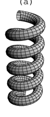
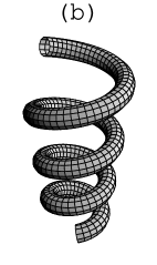
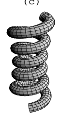
Figure 1: Helical solutions of the Kirchhoff equations using the Lancret’s Theorem. (a) circular helix solution for an inhomogeneous rod with constant bending coefficient $B_{a}=1$ (47); (b) and (c) Lancret helices for inhomogeneous rod with bending coefficient given by Eqs. (48) and (49), respectively. The parameters, in scaled units, are $M_{3}=0.05$, $\Gamma=0.9$, and the total length of the rod is $L=130$. $k_{F}(0)=0.24$ for the helical solutions displayed in panels (a) and (b), and $k_{F}(0)=0.22$ for panel (c).

Figure 2: (a), (b) and (c) are projected curves of the helical solutions displayed in Fig. 1a, Fig. 1b and Fig. 1c, respectively. We used Eq. (13) to obtain the projected curves.

Figure 3: $g_{\lambda}(s)$ for the free standing helix solution displayed in Fig. 1b.

References

- [1] T. Schlick, Curr. Opin. Struct. Biol. 5 (1995) 245. W. K. Olson, Curr. Opin. Struct. Biol. 6 (1996) 242.
- [2] C. W. Wolgemuth, T. R. Powers, R. E. Goldstein, Phys. Rev. Lett. 84 (2000) 1623.
- [3] D. N. McIlroy, D. Zhang, Y. Kranov, M. Grant Norton, Appl. Phys. Lett. 79 (2001) 1540.
- [4] A. Goriely, M. Tabor, Phys. Rev. Lett. 80 (1998) 1564; A. Goriely, M. Tabor, Physicalia 20 (1998) 299.
- [5] T. McMillen, A. Goriely, J. Nonlin. Sci. 12 (2002) 241.
- [6] P. Pieranski, J. Baranska, A. Skjeltorp, Eur. J. Phys. 24 (2004) 613.
- [7] M. Nizette, A. Goriely, J. Math. Phys. 40 (1999) 2830.
- [8] M. P. do Carmo, Differential Geometry of Curves and Surfaces, Prentice Hall, Inc. Englewood Cliffs, New Jersey, 1976.
- [9] D. J. Struik, Lectures on Classical Differential Geometry, 2nd Edition, Addison-Wesley, Cambridge, 1961.
- [10] G. Kirchhoff, J. Reine Anglew. Math. 56 (1859) 285.
- [11] E. H. Dill, Arch. Hist. Exact. Sci. 44 (1992) 2; B. D. Coleman, E. H. Dill, M. Lembo, Z. Lu, I. Tobias, Arch. Rational Mech. Anal. 121 (1993) 339.
- [12] G. H. M. van der Heijden, J. M. T. Thompson, Nonlinear Dynamics 21 (2000) 71.
- [13] S. Neukirch, M. E. Henderson, J. Elasticity 68 (2002) 95.
- [14] I. Tobias, D. Swigon, B.D. Coleman, Phys. Rev. E 61 (2000) 747; B.D. Coleman, D. Swigon, I. Tobias, Phys. Rev. E 61 (2000) 759.
- [15] Y. Sun, J. W. Leonard, Ocean. Eng. 25 (1997) 443; O. Gottlieb, N. C. Perkins, ASME J. Appl. Mech. 66 (1999) 352.
- [16] A. F. da Fonseca, D. S. Galvão, Phys. Rev. Lett. 92 (2004) art. no. 175502.
- [17] A. Mielke, P. Holmes, Arch. Rational Mech. Anal. 101 (1988) 319.
- [18] M. A. Davies, F. C. Moon, Chaos 3 (1993) 93.
- [19] G. Domokos, P. Holmes, Int. J. Non-Linear Mech. 28 (1993) 677.
- [20] G. Domokos, P. Holmes, B. Royce, J. Nonlinear Sci. 7 (1997) 281.
- [21] P. Holmes, G. Domokos, J. Schmitt, I. Szeberényi, Comput. Methods Appl. Mech. Engrg. 170 (1999) 175.
- [22] A. F. da Fonseca, C. P. Malta, M. A. M. de Aguiar, Physica A 352 (2005) 547.
- [23] A. F. da Fonseca, M. A. M. de Aguiar, Physica D 181 (2003) 53.
- [24] A. F. Fonseca, M. A. M. de Aguiar, Phys. Rev. E 63 (2001) art. no. 016611.
- [25] A. Goriely, T. McMillen, Phys. Rev. Lett. 88 (2002) art. no. 244301.
- [26] A whip is a nonhomogenous thread with varying radius of cross section.
- [27] H. Kashimoto, A. Shiraishi, J. Sound and Vibration 178 (1994) 395.
- [28] J. M. T. Thompson, A. R. Champneys, Proc. R. Soc. London, Ser. A 452 (1996) 117.
- [29] A. Goriely, M. Tabor, Nonlinear Dynamics 21 (2000) 101.
- [30] A. Goriely, M. Tabor, Proc. R. Soc. London, Ser. A 453 (1997) 2583.
- [31] A. Goriely, P. Shipman, Phys. Rev. E 61 (2000) 4508.
- [32] G. H. M. van der Heijden, J. M. T. Thompson, Physica D 112 (1998) 201.
- [33] A. Goriely, M. Nizette, M. Tabor, J. Nonlinear Sci. 11 (2001) 3.
- [34] N. Chouaïeb, PhD Thesis, École Polytechnique Fédérale de Lausanne, 2003.
- [35] W. A. Kronert et al, J. Mol. Biol. 249 (1995) 111.
- [36] V. Geetha, Int. J. Biol. Macromol. 19 (1996) 81.
- [37] B. de Saint Venant, J. Ec. Polyt. 30 (1845) 26.
- [38] The references in [11] can be seen for a complete derivation of the Kirchhoff equations.
- [39] J. Langer, D. A. Singer, SIAM Rev. 38 (1996) 605.
- [40] P. Holmes, G. Domokos, G. Hek, J. Nonlinear Sci. 10 (2000) 477.