Active control of sound inside a sphere via control of the acoustic pressure at the boundary surface

Abstract

Here we investigate the practical feasibility of performing soundfield reproduction throughout a three-dimensional area by controlling the acoustic pressure measured at the boundary surface of the volume in question. The main aim is to obtain quantitative data showing what performances a practical implementation of this strategy is likely to yield. In particular, the influence of two main limitations is studied, namely the spatial aliasing and the resonance problems occurring at the eigenfrequencies associated with the internal Dirichlet problem. The strategy studied is first approached by performing numerical simulations, and then in experiments involving active noise cancellation inside a sphere in an anechoic environment. The results show that noise can be efficiently cancelled everywhere inside the sphere in a wide frequency range, in the case of both pure tones and broadband noise, including cases where the wavelength is similar to the diameter of the sphere. Excellent agreement was observed between the results of the simulations and the measurements. This method can be expected to yield similar performances when it is used to reproduce soundfields.

,

1 Introduction

During the last few decades, considerable attention has been paid to soundfield reproduction, which raised many issues in acoustics and signal processing. Several methods can be used to reproduce a given soundfield, the most popular of which are the binaural techniques [1], Ambisonics [2], and Wave Field Synthesis [3]. For a given application, the choice of method will depend on the physical properties of the sound to be reproduced and on the number of listeners.

We focus here in particular on the reproduction of very low frequency soundfields. One of the practical applications of reproducing soundfields of this kind is the perceptual assessment of sonic boom sounds. It is particularly difficult to choose a suitable method of reproducing these soundfields because of their spectral properties: most of the energy of which sonic boom sounds consist involves frequencies below a few dozen Hz, and the spectrum is maximum at only a few Hz [4, 5]. Besides, the acoustic pressure level of sonic booms is often as high as $120$ dB.

More generally, reproducing low-frequency soundfields is of interest for the study of hearing. Perceptual assessments such as those focusing on the inconvenience associated with transport noise are usually performed using headphones. This is the simplest and cheapest method available to deliver a desired soundfield to the ears of a listener. However, this method is not suitable for reproducing very low frequencies, which are thought to be perceived not only by the ears themselves, but by the entire body. The soundfields therefore have to be extended spatially so that they surround at least the listener’s head and torso.

Contrary to binaural techniques, Wave Field Synthesis (WFS) and Ambisonics both give a suitably large reproduction zone surrounding the listener. However, the main problem on which Ambisonics focuses is not so much to accurately reproduce soundfields, but to give the listener a realistic spatial feeling. The principle on which the method is based involves several psychoacoustic hypotheses, which raises problems in the case of infrasonic sounds since the hearing mechanisms mobilised at these frequencies have not yet been completely elucidated. Unlike Ambisonics, WFS focuses on reproducing the physical properties of soundfields in a wide spatial area. Unfortunately, this technique was originally unable to compensate for the reflective properties of the sound reproduction room, whereas reproducing sonic booms requires using a small room to reach the pressure levels required at such low frequencies. Recent studies [6, 7] have shown that a preliminary equalization step can be used to correct the errors induced in WFS by room reflections. However the procedures proposed for this purpose are open-loop ones, which means that the performances of the system can be affected by any change in the physical properties of the reproduction room, such as temperature changes.

Several sound reproduction methods have been proposed since the nineties, based on active noise control strategies. Cancelling a primary noise is basically the same task as reproducing it, since a perfect cancellation of the primary noise requires generating a secondary noise which has exactly the same properties, apart from they are in opposition of phase. The main advantage of methods of this kind is that they can be used to compensate for the reflections generated in the reproduction room by means of adaptive filters. Some of these “active control” methods can be compared with local active noise control strategies [8, 9, 10, 11, 12, 13, 14]. With these methods, either error microphones are placed directly in the area where the soundfield is to be reproduced, or preliminary measurements are carried out to design control filters. The presence of microphones in the reproduction area is not advisable because these conditions may be uncomfortable for the listener. In addition, in order to reproduce a soundfield in a three dimensional area, a very large number of sensors can be required. On the other hand, as with WFS, the use of an off-line filter design prevents the performances of the system from remaining constant when the acoustical properties of the reproduction room fluctuate.

Another category of “active control” soundfield reproduction methods is based on the application of the Kirchhoff-Helmholtz integral formula [15, 16, 17, 18]. In particular, the Boundary Pressure Control technique (BPC) [16] is based on the assumption that the acoustic pressure inside a given volume depends only on the pressure on the boundary surface, excepted at certain frequency values. Secondary sources generate a soundfield which is measured by microphones placed on the boundary surface of the volume, and then compared with the soundfield to be reproduced. BPC can be used to reproduce a given soundfield over a spatially extended area free of microphones, and enables to accurately compensate for the room reflections using adaptive filtering methods. This approach therefore seems to be appropriate for reproducing low-frequency soundfields.

In this paper, the results of a feasibility study on the application of BPC to low-frequency soundfield reproduction are presented. In order to quantify the performances that can be expected when this strategy is used, application of BPC to active noise control in free field was tested, both numerically and experimentally. The reason why this has not been done before is probably that the implementation of this sound control strategy requires the use of many sensors and actuators, which have to be managed by one or several high-performance multichannel electronic controllers. Although the results presented in this paper have been obtained in the context of active noise control, similar performances could probably be obtained in that of soundfield reproduction, since cancelling a noise and reproducing it constitute basically the same physical task. Besides, the same hardware and algorithms can be used in both tasks with very few changes [19].

In the paper, the theory of BPC and its practical limitations are presented in section 2. Numerical BPC simulations in the time and frequency domains are presented in section 3. The experimental results obtained after real-time implementation of BPC are given in section 4. An excellent agreement was observed between the results of the simulations and of the measurements, which make possible in the end the statement of practical design rules for sound reproduction through BPC.

2 Active control of sound using the Boundary Pressure Control method

2.1 Kirchhoff–Helmholtz equation

The Boundary Pressure Control technique involves the integral representation of the acoustic field. As shown in Fig. 1, let $\Omega$ denote a volume in space and $\Sigma$ its boundary surface. If there is no acoustic source inside $\Omega$, then the pressure at any point $\mathrm{\bf{r}}_{\Omega}$ in $\Omega$ (but not on $\Sigma$) can be written as [20]:

$$p(\mathrm{\bf{r}}_{\Omega})=\int\!\!\!\int_{\Sigma}\left(G(\mathrm{\bf{r}}_{\Omega},\mathrm{\bf{r}}_{\Sigma})\frac{\partial p(\mathrm{\bf{r}}_{\Sigma})}{\partial\mathrm{\bf{n}}_{\Sigma}}-p(\mathrm{\bf{r}}_{\Sigma})\frac{\partial G(\mathrm{\bf{r}}_{\Omega},\mathrm{\bf{r}}_{\Sigma})}{\partial\mathrm{\bf{n}}_{\Sigma}}\right)\mathrm{d\bf{r}}_{\Sigma}$$ (1)

where $G$ is the Green’s function in free space, and $\mathrm{\bf{n}}_{\Sigma}$ the unit vector normal to the surface. This integral representation of the acoustic pressure, known as the Kirchhoff–Helmholtz equation, shows that the acoustic pressure measured inside a volume depends only on the pressure and its normal derivative measured over the whole surface enclosing the volume. Moreover, for a point $\mathrm{\bf{r}}_{\Omega}$ that lies on the boundary $\Sigma$, it can be shown that [20]:

$$\frac{1}{2}p(\mathrm{\bf{r}}_{\Sigma}^{0})=\int\!\!\!\int_{\Sigma}\left(G(\mathrm{\bf{r}}_{\Sigma}^{0},\mathrm{\bf{r}}_{\Sigma})\frac{\partial p(\mathrm{\bf{r}}_{\Sigma})}{\partial\mathrm{\bf{n}}_{\Sigma}}-p(\mathrm{\bf{r}}_{\Sigma})\frac{\partial G(\mathrm{\bf{r}}_{\Sigma}^{0},\mathrm{\bf{r}}_{\Sigma})}{\partial\mathrm{\bf{n}}_{\Sigma}}\right)\mathrm{d\bf{r}}_{\Sigma}$$ (2)

In addition to Eq. (1), Eq. (2) means that there exists a linear relation between the pressure and its normal derivative, both measured on $\Sigma$. The pressure inside $\Omega$ therefore depends only on the pressure measured on its boundary surface. The general idea underlying the Boundary Pressure Control technique is that one needs to impose the appropriate pressure value only over the whole boundary surface to obtain the required soundfield anywhere inside the volume. To reproduce of a given soundfield, the method consists in: 1. recording the acoustic pressure over the whole surface of the volume; 2. reproducing the same pressure values at the points where they were recorded. Another way of interpreting Eqs. (1) and (2) means that BPC can be used for active noise control: with these equations, it is only necessary to cancel the acoustic pressure only over the whole boundary surface to cancel it anywhere inside the volume.

2.2 Practical limitations of BPC

Unfortunately, the use of the BPC technique has two serious limitations. The first one, which is commonly known as spatial aliasing, is due to the spatial undersampling of the surface controlled. Eqs. (1) and (2) are integral representation of the soundfield, which involve summing up the values of the pressure and its normal derivative on a continuous distribution of points over the whole surface under consideration. In practice, this would involve controlling the soundfield at an infinite number of points, which is of course impossible. Actually, in the practical implementation of either a soundfield reproduction or an active noise control system, it will not be possible to monitor the sound at more that a few dozen points, and the performances of the system will therefore decrease when the frequency increases [8, 21].

The second physical limitation results from the mathematical properties of Eq. (2). Assuming that the pressure is equal to zero all over $\Sigma$, Eq. (2) becomes

$$\int\!\!\!\int_{\Sigma}\left(G(\mathrm{\bf{r}}_{\Sigma}^{0},\mathrm{\bf{r}}_{\Sigma})\frac{\partial P(\mathrm{\bf{r}}_{\Sigma})}{\partial\mathrm{\bf{n}}_{\Sigma}}-P(\mathrm{\bf{r}}_{\Sigma})\frac{\partial G(\mathrm{\bf{r}}_{\Sigma}^{0},\mathrm{\bf{r}}_{\Sigma})}{\partial\mathrm{\bf{n}}_{\Sigma}}\right)\mathrm{d\bf{r}}_{\Sigma}=0$$ (3)

Finding the solutions to Eq. (3) is known as the interior Dirichlet problem. Eq. (3) has an infinite number of solutions when the frequency is equal to some eigenvalues depending on the shape of the surface [22]. For example, in the case of a rectangular parallelepiped, the corresponding frequency values are given by

$$f_{\mathrm{lmn}}=\frac{c}{2}{\sqrt{{\left(\frac{l}{L_{\mathrm{x}}}\right)}^{2}+{\left(\frac{m}{L_{\mathrm{y}}}\right)}^{2}+{\left(\frac{n}{L_{\mathrm{z}}}\right)}^{2}}}$$ (4)

where $l$, $m$ and $n$ are strictly positive integers and $L_{\mathrm{x}}$, $L_{\mathrm{y}}$ and $L_{\mathrm{z}}$ are the dimensions of the parallelepiped. In the case of a spherical volume, the characteristic wave numbers correspond to the zeros of the spherical Bessel functions. In particular, the values

$$f_{\mathrm{k}}=k\frac{c}{2r}$$ (5)

are eigenfrequencies of the problem, where $k$ is a positive integer, $r$ the radius of the sphere and $c$ the celerity of sound. It is easy to show that Eq. (2) also has an infinite number of solutions at these frequencies. In practice, this means that if the acoustic pressure is made to be equal to the appropriate value all over $\Sigma$, it will not necessarily be equal to the appropriate value inside $\Omega$ if the frequency is equal to one of the eigenfrequencies of the interior Dirichlet problem related to $\Omega$.

In parts 3 and 4, the feasibility of soundfield reproduction using BPC is studied via simulations and active noise cancellation experiments inside a sphere. The sphere was chosen because, among the various shapes with the same capacity $V$, the sphere is the shape with the lowest surface value. When performing active noise control inside a volume with capacity $V$ using a BPC strategy, the sphere therefore gives the best spatial discretization of the boundary surface with a given number of minimisation microphones. In addition, the sphere is the most regular shape possible: the resonances resulting from the singularity in the Dirichlet problem are therefore expected to be maximum in this case, so that they can be easily detected. As far as the authors know, these resonances have never been studied experimentally in the field of active noise control or sound reproduction, because this requires the use of a sufficiently large number of transducers, depending on the shape of the volume in which the control is to be carried out. Preliminary simulations showed that in the case of a sphere, about $16$ microphones are required, whereas in the case of a cube, at least $50$ microphones are required, which is a heavy constraint for active noise control implementations.

2.3 From active noise control to soundfield reproduction

Let us consider an active noise control setup, including a number of primary sources, secondary sources and minimisation microphones. In the frequency domain, each acoustic path between a source and a microphone is entirely described by a complex scalar. If $\mathrm{\bf{G}}$ denotes the matrix of the acoustic paths between the secondary sources and the minimisation microphones, and $\mathrm{\bf{p}}_{0}$ the vector of the primary pressures measured at the microphones, then the vector of optimal command signals for noise cancellation with the secondary sources, regardless of any causality or feasibility constraint, is given by:

$$\mathrm{\bf{u}}=-{\mathrm{\bf{G}}}^{-1}{\mathrm{\bf{p}}}_{0}$$ (6)

If Tikhonov regularization [23] is introduced into the matrix inversion process, which corresponds to adding an effort weighting to the command vector computation [24], Eq. (6) becomes

$$\mathrm{\bf{u}}=-{(\mathrm{\bf{G}}^{\mathrm{H}}\mathrm{\bf{G}}+\beta I)}^{-1}\mathrm{\bf{G}}^{\mathrm{H}}{\mathrm{\bf{p}}}_{0}$$ (7)

where $\beta$ is the regularization coefficient. Such a coefficient usually helps in widening the minimisation area around the microphones because with regularization the noise minimisation problem at a finite number of microphones fits better the underlying global minimisation problem at an infinite number of locations. Therefore, if $\mathrm{\bf{H}}$ denotes the matrix of acoustic paths between the secondary sources and some observation points, the total pressure $\mathrm{\bf{p}}_{\mathrm{tot}}$ measured at these points when the control is on is given by the formula

$${\mathrm{\bf{p}}}_{\mathrm{tot}} = {\mathrm{\bf{p}}}_{\mathrm{pri}}+{\mathrm{\bf{p}}}_{\mathrm{sec}}$$ (8)

$$= {\mathrm{\bf{p}}}_{\mathrm{pri}}+{\mathrm{\bf{H}}}\mathrm{\bf{u}}$$

$$= {\mathrm{\bf{p}}}_{\mathrm{pri}}-\mathrm{\bf{H}}{(\mathrm{\bf{G}}^{\mathrm{H}}\mathrm{\bf{G}}+\beta I)}^{-1}\mathrm{\bf{G}}^{\mathrm{H}}{\mathrm{\bf{p}}}_{0}$$

where ${\mathrm{\bf{p}}}_{\mathrm{pri}}$ is the vector of pressures when the control is off, and ${\mathrm{\bf{p}}}_{\mathrm{sec}}$ denotes the vector of secondary pressures, both measured at the observation points. The mean attenuation obtained on $N$ observation points ($\mathrm{\bf{x}}_{1}$, $\mathrm{\bf{x}}_{2}$, … $\mathrm{\bf{x}}_{\mathrm{N}}$) can then be written:

$$A=\frac{1}{N}\sum\limits_{k=1}^{N}20{log}_{10}\left|\frac{{\mathrm{\bf{p}}}_{pri}(\mathrm{\bf{x}}_{\mathrm{k}})}{{\mathrm{\bf{p}}}_{tot}(\mathrm{\bf{x}}_{\mathrm{k}})}\right|$$ (9)

Let us now consider the case where the same arrangement of sources and microphones is used for soundfield reproduction purposes. The task now consists in generating a soundfield with the secondary sources which is as similar as possible to the primary soundfield at the minimisation microphones. The vector of optimal command signals with regularization is given here by:

$$\mathrm{\bf{u}^{\prime}} = {(\mathrm{\bf{G}}^{\mathrm{H}}\mathrm{\bf{G}}+\beta I)}^{-1}\mathrm{\bf{G}}^{\mathrm{H}}{\mathrm{\bf{p}}}_{0}$$ (10)

$$= -\mathrm{\bf{u}}$$

Hence, the vector of the reproduced pressures, which is also the vector of the secondary pressures measured at the observation points, is given by:

$${\mathrm{\bf{p}}}_{\mathrm{sec}}^{\prime}=-{\mathrm{\bf{p}}}_{\mathrm{sec}}$$ (11)

Whereas the attenuation is the most appropriate criterion for assessing the noise control performances, the quality of the reproduction can be measured in terms of relative error:

$$E=\frac{1}{N}\sum\limits_{k=1}^{N}20{log}_{10}\left|\frac{{\mathrm{\bf{p}}}_{\mathrm{pri}}(\mathrm{\bf{x}}_{\mathrm{k}})-{\mathrm{\bf{p}}}_{\mathrm{sec}}^{\prime}(\mathrm{\bf{x}}_{\mathrm{k}})}{{\mathrm{\bf{p}}}_{\mathrm{pri}}(\mathrm{\bf{x}}_{\mathrm{k}})}\right|$$ (12)

Replacing ${\mathrm{\bf{p}}}_{\mathrm{sec}}^{\prime}$ in Eq. 12 by the value given in Eq. 11, we obtain:

$$E = \frac{1}{N}\sum\limits_{k=1}^{N}20{log}_{10}\left|\frac{{\mathrm{\bf{p}}}_{\mathrm{pri}}(\mathrm{\bf{x}}_{\mathrm{k}})+{\mathrm{\bf{p}}}_{\mathrm{sec}}(\mathrm{\bf{x}}_{\mathrm{k}})}{{\mathrm{\bf{p}}}_{\mathrm{pri}}(\mathrm{\bf{x}}_{\mathrm{k}})}\right|$$ (13)

$$= \frac{1}{N}\sum\limits_{k=1}^{N}20{log}_{10}\left|\frac{{\mathrm{\bf{p}}}_{\mathrm{tot}}(\mathrm{\bf{x}}_{\mathrm{k}})}{{\mathrm{\bf{p}}}_{\mathrm{pri}}(\mathrm{\bf{x}}_{\mathrm{k}})}\right|$$

$$= -A$$

The reconstruction error is therefore the opposite of the attenuation obtained in the case of active noise cancellation. In other words, if the active noise control setup attenuates a given noise of $40$ dB, it will be able to reproduce the primary soundfield pressure with a relative error of $-40$ dB, e.g. $1$ %.

Assuming that the acoustic paths are the same in both cases, the optimum active noise control and soundfield reproduction performances will be similar in the frequency domain, which is quite natural, since in both cases, the performances depend only on the inversion of the matrix of secondary acoustic paths. For the same reasons, the performances of noise cancellation and reproduction will also be similar using adaptive algorithms in the time domain. It is therefore possible to assess the performances of a soundfield reproduction setup using it as an active noise control setup, and vice-versa.

3 Numerical simulations

3.1 The setup used in simulations

In this section, the results of preliminary numerical simulations performed in the case of the $30\times 30$ multi-channel active noise control of a spherical volume are presented. It was proposed here to simulate the behaviour of an active noise control setup in order to compare the results with those obtained experimentally (part 4). However, it is worth noting that the results would be exactly the same if the setup simulated was a soundfield reproduction system, as shown in section 2.3. Firstly, the system was simulated in the frequency domain in order to determine the optimum predictable attenuation. The results obtained were most encouraging, although the two limitations mentioned in part 2 dramatically restricted the noise cancellation performances inside the volume. Secondly, the system was simulated in the time domain in order to assess the performances of a real system involving a Filtered-X Least Mean Square (FXLMS) time-domain algorithm. Two types of primary fields were tested: pure tones, and broadband noises. The results were predictably less satisfactory here than in the frequency-domain case, because it was difficult to make the algorithm converge. An interesting finding which emerged was the fact that the problem of Dirichlet resonances is a serious weakness of the system even in the case of a broadband primary soundfield.

Figs. 2 and 3 show the setup used in the numerical simulations. It was composed of one virtual primary source, $30$ virtual secondary sources, and $30$ minimisation microphones. As shown in Fig. 2, the virtual microphones were distributed on the surface of a sphere with a diameter of $30$ cm, along $8$ arcs of a circle, as far from each other as possible. The positions of the secondary sources were the homothetical images of the microphone positions on a sphere with a radius of $60$ cm radius. The primary source was located on the same horizontal plane as the center of the sphere, $4$ m away from it. In the computations, all the transducers were assumed to be perfect monopoles in free field: therefore, the impulse responses of each source measured at each microphone were perfect impulses with a time-delay of $\frac{r}{c}$ seconds, attenuated by a factor $r$, where $r$ denotes the distance between the transducers.

3.2 Frequency-domain simulations

Frequency-domain simulations were carried out using the optimal control formulation given in section 2.3. Fig. 4 shows the average attenuation obtained with a mesh consisting of $160$ points regularly spaced inside the sphere as a function of the frequency, without any regularisation procedure ($\beta=0$ in Eq. 7). This figure illustrates the two physical limitations mentioned in part 2. In a first approximation, it can be seen that the average attenuation decreased linearly from $0$ to $1000$ Hz, by approximately $6$ dB per Hz. This regular decrease in the control performances was due to the spatial undersampling: the higher the frequency, the less satisfactory the discretization of the soundfield over the boundary surface and the control performance became. In addition, the control performances dropped dramatically when the frequency of the primary soundfield approached the eigenfrequencies of the interior Dirichlet problem. The attenuation even fell to less than $-30$ dB, which means that the interior pressure level present when the control was on was more than ten times that occurring when control was off. This was because only the acoustic pressure was controlled, although both the pressure and its normal derivative should be controlled: the sound pressure can have any value inside the sphere, even if the control is highly efficient at the level of the minimisation microphones.

Fig. 5 shows the results obtained in the case where $\beta$ was taken to be equal to $0.9$. It shows that it is possible to prevent the pressure attenuation from being negative at the eigenfrequencies of the Dirichlet problem by regularizing the matrix before it is inverted. This improvement is achieved with no great loss in the control performances inside the sphere, as shown in Fig. 6. Another advantage of the regularization procedure is that it decreases the amplitude of the command vector. This suggests that in the time domain, it might be useful to add a leakage term to the control algorithm [24], which is similar to performing Tikhonov regularization in the frequency domain and can usefully increase the stability of an active noise control system of this kind. Note that in the case of a regularized matrix inversion process, the attenuation observed inside the sphere can be greater than that observed at the minimisation microphones.

3.3 Time-domain simulations

In the time domain, the acoustic paths between each source and each microphone are described by impulse responses. In the case of perfect point sources under free-field conditions, the impulse responses are time-delayed, attenuated pulses. However, since the time delays are mostly not exact numbers of sampling periods, the impulse responses need to be approximated for discrete-time simulation purposes. The accuracy of the approximation depends strongly on the sampling frequency. In this study the frequency chosen was $8192$ Hz, which has been found to suffice in view of the dimensions of the setup: the shortest distance between two transducers was $30$ cm, which corresponds to a delay of approximately $7$ samples at this frequency. The transfer functions were first computed in the frequency domain in $8192$ frequency bins, and they were then converted into impulse responses by performing an Inverse Fast Fourier Transform (IFFT) and truncated to their first $256$ coefficients. The impulse responses obtained were finally used in a program simulating a multichannel FXLMS algorithm in the time domain. The same formulation as in [24] was used to adapt the filter coefficients:

$$\mathrm{\bf{w}}(n+1)=\mathrm{\bf{w}}(n)-\alpha\left(\hat{\mathrm{\bf{R}}}^{\mathrm{T}}(n)\mathrm{\bf{e}}(n)+{\beta}^{\prime}\mathrm{\bf{w}}(n)\right)$$ (14)

where $\mathrm{\bf{w}}(n)$ denotes the vector of the minimisation filter coefficients at the $n$th sample time, $\hat{\mathrm{\bf{R}}}(n)$ denotes the matrix of the estimated filtered reference signals, $\mathrm{\bf{e}}(n)$ denotes the vector of the error signals, $\alpha$ denotes the convergence coefficient, and ${\beta}^{\prime}$ is a regularization coefficient. Note that the primary source command signal was used as the reference signal by the FXLMS algorithm. Two types of simulation were carried out, corresponding to two types of primary signals: firstly, a pure tone signal at various frequencies; and secondly, a broadband signal with a frequency range of $0$–$900$ Hz.

In the case of pure tone primary signals, the frequency was increased step by step: at each frequency value, the algorithm was let to converge during a few thousand samples, and the value of the attenuation was then averaged based on the last thousand samples and saved. Note that the $\alpha$ convergence coefficient was the same at each frequency value. As in the experimental case, the length of the estimated secondary paths was $200$ coefficients and the length of the minimisation filters was $10$ coefficients. Fig. 7 shows the pressure attenuation obtained with pure tone primary signals from $200$ to $1000$ Hz at the minimisation microphones, compared to the averaged pressure attenuation inside the sphere. The results obtained here were very similar to those obtained in the frequency domain in the regularized case throughout the frequency band, but the control was less efficient in the time domain. The attenuation is not shown here at frequencies inferior to $200$ Hz, because the algorithm had difficulty in converging at lower frequencies, and the computation time required for the algorithm to converge with a smaller value of the $\alpha$ coefficient would have been too long. This convergence problem results from the ill-conditioning of the matrix of secondary paths at low frequencies [21], which again confirms the importance of using leakage in systems of this kind.

In the case of a broadband primary signal, the length of the minimisation filters and estimated secondary paths were both set at $90$ coefficients. The algorithm was made to converge during several dozen thousands of samples, and the minimisation filters obtained were then used to compute in the frequency domain the pressure attenuation occurring inside the sphere and at the minimisation microphones. Fig. 8 shows the control performances obtained using this method with leakage in the case of a $0$–$900$ Hz white primary noise. Similar findings to those made in the case of pure tone signals can be obtained here: although the control performances observed at the minimisation microphones are good throughout the frequency range of the primary signal, the average pressure attenuation obtained inside the volume becomes poor at frequencies approaching the eigenvalues of the Dirichlet problem. Note that for frequencies below $500$ Hz, the performances obtained inside the sphere were more satisfactory than those obtained at the minimisation microphones.

3.4 Conclusions

Several important conclusions can be drawn from this preliminary study. First, all the simulations presented here showed how efficiently the system controls low-frequency noise. The control performances were satisfactory throughout the volume at frequencies below $500$ Hz in all the cases tested. At this frequency, the wavelength is $68$ cm, which is approximately equal to the diameter of the sphere: the control is therefore no longer local and actually includes the whole volume. Secondly, the inaccuracy of the spatial sampling and the non-uniqueness of the interior Dirichlet problem seem to be two important limitations of this control method, including for control of broadband noises. Thirdly, leakage appears to be a useful means of reducing the resonance problems which occur when the frequency tends to the eigenvalues of the Dirichlet problem.

4 Experiments

4.1 Experimental setup

Although the aim of this study was to investigate the feasibility of soundfield reproduction using BPC, we decided to assess the setup performances by performing active noise control experiments using the same strategy. The controllers used here had already been programmed with an active noise control algorithm, and the behaviour of the setup was expected to be similar in the case of both active noise cancellation soundfield reproduction, as shown in part 2.3.

The setup used in these experiments is shown in Fig. 9. Thirty minimisation microphones were distributed over the whole surface of a sphere with a diameter of $60$ cm, as in the case of the setup modelled in the numerical simulations. The primary soundfield was emitted by a primary loudspeaker placed at a few meters from the microphone sphere, and was controlled by thirty secondary sources distributed over the surface of a sphere with a diameter of $170$ cm, so that the distance between each secondary source and the nearest minimisation microphone was approximately $30$ cm. Secondary sources and minimisation microphones were numbered so that microphone $1$ was the nearest microphone to source $1$, and so on. In addition to the minimisation microphones, two other microphones were placed inside the microphone sphere in order to measure the control performances inside the sphere: one was in the center, and the other one was approximately mid-way between the center of the sphere and its surface. As in the numerical simulations, the control performances were measured in the case of two types of primary noises: pure tone noise, and broadband noise.

In the case of the pure tone noise, the secondary source command signals were computed by a $32\times 32$ multichannel controller designed for active control of tonal disturbances. The secondary paths identified were saved into FIR filters with $200$ coefficients and the length of the minimisation FIR filters was arbitrarily chosen as $10$ coefficients, although $2$ coefficient may have sufficed in theory. The frequency of the primary sound was increased by $5$ Hz every $16$ s from $200$ to $700$ Hz: the algorithm was let to converge during the first $8$ s and the acoustic pressure was measured during the last $8$ s. The convergence coefficient $\alpha$ remained constant throughout the measurement process. In both the measurement process and the control process, the sampling frequency was $2048$ Hz.

In the case of broadband noise, however, secondary source command signals were computed by two $16\times 16$ multichannel LMA COMPARS controllers [25] programmed with an FXLMS algorithm, as shown in Figs. 10 and 11. The inputs to the first COMPARS were the pressure signals from microphones $1$–$16$, and the outputs were the secondary sources $1$–$16$ command signals; the second COMPARS received the signals from microphones $17$–$30$, and computed the commands to be transmitted to sources $17$–$30$. Note that the microphones and sources were spatially distributed in two blocks in order to ensure the simultaneous convergence of the both algorithms. The whole active noise control setup, including the two controllers, can be viewed in fact as a single FXLMS system with a block-diagonal matrix of identified secondary paths: a sufficient condition for this system to converge is that the matrix of real secondary paths is block-diagonal dominant [26]. Note also that the experiment was conducted in a quasi-anechoic environment to facilitate the convergence of the algorithms. If the system had been implemented in a more reverberant room, the reflections from the walls would have increased the effects of each secondary source on the distant minimisation microphones, and the transfer matrix would have been less diagonally dominant. Lastly, the electric signal fed to the primary source was used by both controllers as a reference signal for the FXLMS algorithm. The identified secondary paths and the control filters both consisted of FIR filters with $90$ coefficients. As in the pure tone case, a sampling frequency of $2048$ Hz was used. The primary noise was therefore a white noise with a $0$ to $1024$ Hz spectrum. The convergence coefficient ($\alpha$ in Eq. 14) was taken to be approximately half of the value at which the algorithm began to diverge and was the same in the two controllers.

4.2 Results in the pure tone case

Fig. 12 shows the attenuation measured at the minimisation and observation microphones in the case of pure tone primary signals with frequency ranging from $100$ to $700$ Hz. In the $200$–$500$ Hz frequency band, the attenuation values measured both on the surface of the sphere and inside it were greater than $30$ dB, which corresponds to a highly efficient control in the whole volume. Beyond $500$ Hz, however, the attenuation dropped off dramatically at the observation microphones, reaching a minimum value of only a few dB at $580$ Hz, although it was still above $30$ dB at the minimisation microphones. Note that the minimum attenuation was obtained when the frequency ranged between $580$ and $590$ Hz, which is slightly above the value of $566$ Hz expected for a sphere with a radius of $30$ cm. However, this amount of frequency shift was more or less expected, because the measured eigenfrequency corresponds to a radius of $29$ cm and $1$ cm was approximately the accuracy of the minimisation microphone localization. Note also that the attenuation decreased at frequencies below $200$ Hz. This was due to two factors: first, the secondary sources used for the noise control were small, and therefore not very powerful at low frequencies; second, the convergence of the algorithm was slow in this frequency range, probably because of the ill-conditioning of the matrix of secondary paths. One interesting result emerged when the attenuation curves of the two interior microphones were compared: the attenuation measured at microphone $1$ when the frequency was close to the first eigenfrequency of the sphere is lower than that measured at microphone $2$. This finding can be explained by the fact that the first eigenmode of the sphere is radial, the maximum pressure value being reached in the center of the sphere, where microphone $1$ was located.

Good agreement was found to exist here between the experimental data and the results of the simulations, as shown in Fig. 13. The value of the sphere radius was set at $29$ cm in the simulation, in order to take into account the shift of the first eigenfrequency observed experimentally: this corresponds to the first eigenfrequency occurring at approximately $585$ Hz. It can be seen from Fig. 13 that even if the assumptions made in the numerical simulations (point sources in free field) are not met in the experiment, the computations give a very good idea of what occurs in practice. On the one hand, the frequency-domain simulations of optimal control give an approximation of the maximum attenuation values reached in the experiments. On the other hand, the values obtained in the time-domain simulations were very similar to those measured in practice, including the differences in the attenuation between the two interior microphones. Note that the minimum attenuation value was obtained at interior microphone $1$, which was placed in the center of the sphere, under both real and simulated conditions.

4.3 Results in the broadband case

Fig. 14 shows the amplitude of the frequency response measured between the primary source command signal and the minimisation microphones in the case of a $0$–$1024$ Hz broadband primary sound, with and without control. As was to be expected the control performances were less satisfactory here than with pure tone signals. However, the control was found to be highly efficient, since the attenuation achieved was above $15$ dB in almost the whole frequency range under consideration. Note that the poor control performances measured at frequencies around $150$ Hz are due to the insufficient electrical insulation between the components of the experimental setup and the power supply.

The control performances obtained inside the sphere are given in Fig. 15. As in the case of pure tone signals, the pressure attenuation achieved inside the sphere was greater than the attenuation at the surface at frequencies below $500$ Hz. Below this frequency, the setup is therefore able to efficiently cancel a random noise anywhere in the sphere. Above this frequency, however, the attenuation decreases inside the sphere, reaching a minimum value of around $0$ dB at a frequency of $585$ Hz. Note that with interior microphone $1$, which is in the center of the sphere, the attenuation is even negative between $570$ and $600$ Hz. The pressure measured at the interior microphone $1$ when the control is on is therefore greater than the pressure measured when the control is off at these frequency values. Note also that the magnitude of the resonance occurring at around $585$ Hz at microphone $1$ is greater than at microphone $2$. This confirms that the resonance induced at this frequency corresponds to a radial eigenmode, which reaches a maximum value in the center of the sphere.

In Fig. 16, the experimental results are compared with those of the simulations. It can be seen that the simulation does not model the experimental setup behaviour above $600$ Hz. However, the agreement between the measured attenuation and the numerically computed values is very good below this frequency. The simulated attenuation values calculated at both the minimisation microphones and the interior microphones are very similar to those obtained in practice. Besides, as in the pure tone case, the differences in noise attenuation at the interior microphones are well reproduced, including the fact that around $585$ Hz the attenuation reaches a minimum in the center of the sphere.

4.4 Conclusions: interpretation in terms of soundfield reproduction

The experimental results obtained with the present active noise control setup can be interpreted in terms of soundfield reproduction, as described in part 2.3. These results show that an attenuation amounting to more than $30$ dB was obtained in the pure tone signals at frequencies below $500$ Hz. The setup is therefore able to reproduce pure tone soundfields in the same frequency range with an error of less than $3$ %, which is very accurate. In the case of broadband noise, the results show that the reconstruction error can reach about $10$ % ($-20$ dB) in the $100-500$ Hz frequency range. These results are most encouraging and show that BPC has considerable potential for use as a low-frequency soundfield reproduction strategy.

However, the negative attenuation observed when Dirichlet resonance occurred suggests the presence of a reconstruction error grater than $100$ %, which means that a reproduction system based on the use of BPC would be completely unable to reproduce soundfields at the eigenfrequencies of the internal Dirichlet problem.

5 General conclusions and perspectives

In this study, it was established that an active noise control setup based on the Boundary Pressure Control technique can efficiently cancel noise everywhere inside a volume. The existence of considerable similarities between active noise control and soundfield reproduction suggests that similar performances can be obtained when BPC is used to reproduce soundfields. However, the results of both simulations and experimental measurements show that spatial aliasing and the non-uniqueness of the solution to the interior Dirichlet problem limit the use of this strategy. In particular, resonance processes occurring inside the volume when the frequency approaches the eigenfrequencies of the Dirichlet problem completely prevent the system from cancelling the primary noise at these frequencies. It was observed that in practice the attenuation can even become negative when these resonances occur. In the case of soundfield reproduction applications, this means that the reconstruction error could be greater than 100 % at these frequencies. Besides, the data obtained here show that the problem occurs in the case of both pure tone signals and broadband noise signals. Thus, finding a means of reducing the drop in the performances resulting from this problem without increasing the number of transducers required would be an interesting goal for future studies. Some solutions have already been proposed in [16] and [15], such as adding a minimisation microphone inside the volume under consideration, but these solutions have not yet been tested in practice, nor in 3D numerical simulations.

This study was carried out in an almost anechoic environment, in order to simplify the impulse responses which had to be compensated by the controller. However, in order to reach high pressure levels at very low frequencies required by a realistic reproduction of sonic booms, the reproduction system has to be implemented in a room, and the reflections occurring under these conditions cannot be neglected. Longer minimisation filters will probably be required to achieve comparable performances in a room, as the impulse responses of the secondary sources will be longer under these conditions than in a quasi-anechoic environment. The numerical simulation of an in-room soundfield reproduction system has been previously carried out [27] and the results suggest systems of this kind can accurately reconstruct low-frequency wavefronts. The authors therefore intend in the future to implement low-frequency soundfield reproduction strategies using BPC in a specially designed reproduction room.

List of figure captions

Fig. 1: Notations for the Kirchhoff–Helmholtz equation
Fig. 2: The microphone arrangement of the simulation setup
Fig. 3: Geometry and dimensions of the simulation setup
Fig. 4: Frequency-domain simulation: average pressure attenuation measured inside the sphere as a function of the frequency, without regularization. The dotted lines mark the two first eigenfrequencies of the interior Dirichlet problem, at $566$ and $816$ Hz.
Fig. 5: Frequency-domain simulation: average pressure attenuation as a function of the frequency, with regularization (  inside the sphere, — at the minimisation microphones)
Fig. 6: Frequency-domain simulation: average pressure attenuation measured inside the sphere as a function of the frequency (  with regularization, — without regularization)
Fig. 7: Time-domain simulation: average pressure attenuation obtained for pure tone signals as a function of the frequency (  inside the sphere, — at the minimisation microphones)
Fig. 8: Time-domain simulation: average pressure attenuation obtained in the case of broadband noise as a function of the frequency (  inside the sphere, — minimisation microphones)
Fig. 9: The experimental setup. On the left: the primary source. On the right: the 30 secondary sources, the 30 minimisation microphones, and the two interior measurement microphones.
Fig. 10: The two COMPARS controllers used in the case of the broadband noise signal.
Fig. 11: Experimental setup used in the case of the broadband noise signal.
Fig. 12: Experimental results: the pressure attenuation measured in the case of for pure-tone primary signals as a function of the frequency (  interior microphone 1, — interior microphone 2, — minimisation microphones)
Fig. 13: Comparison between simulation and experimental results, in the case of pure-tone primary signals: (a) average attenuation at the minimisation microphones, (b) interior microphone 1, (c) interior microphone 2 (— experiment, — time-domain simulation, $\cdots$ frequency-domain simulation)
Fig. 14: Experimental results: magnitude of the frequency response measured between the primary source command and the minimisation microphones in the case of a broadband noise primary signal (  control on, — control off)
Fig. 15: Experimental results: pressure attenuation measured with a broadband noise primary signal as a function of the frequency (  interior microphone 1, — interior microphone 2, — minimisation microphones)
Fig. 16: Comparison between simulation and experimental results, in the case of a broadband noise primary signal: (a) average attenuation at the minimisation microphones, (b) interior microphone 1, (c) interior microphone 2 (  experiment, — simulation)

Figure 1:

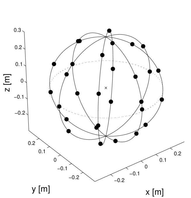
Figure 2:

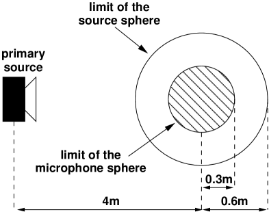
Figure 3:

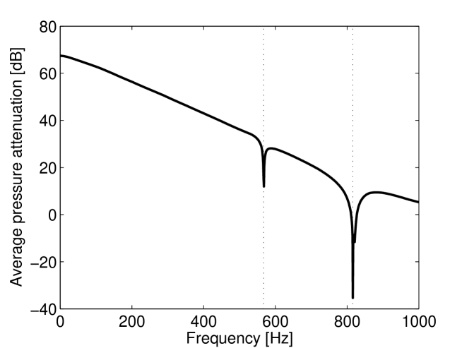
Figure 4:

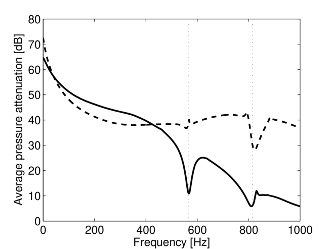
Figure 5:

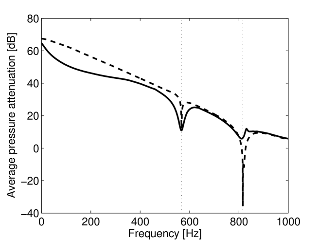
Figure 6:

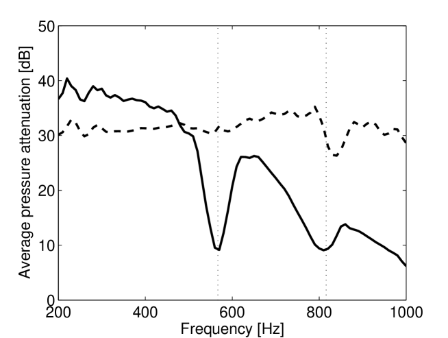
Figure 7:

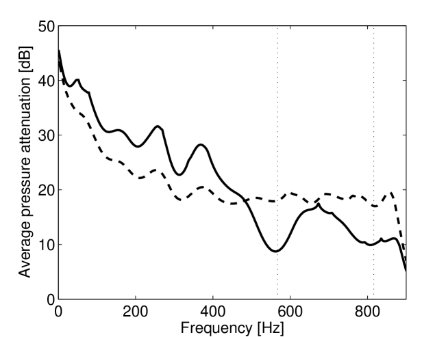
Figure 8:

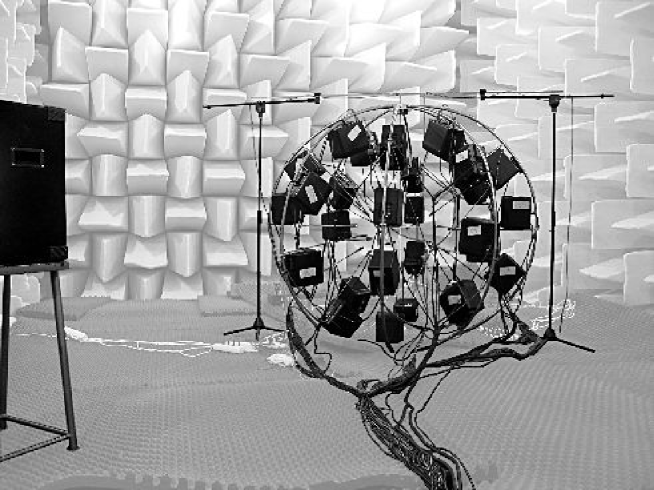
Figure 9:

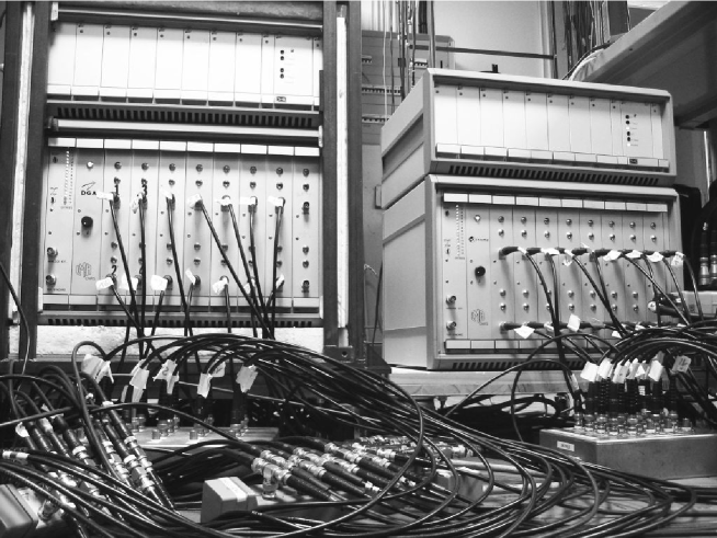
Figure 10:

Figure 11:

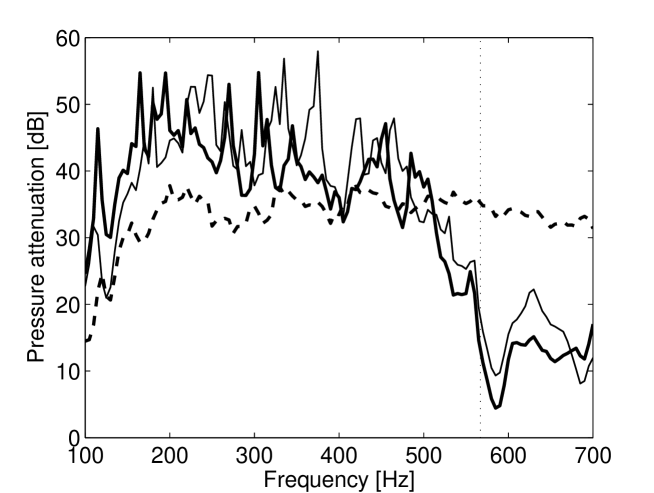
Figure 12:

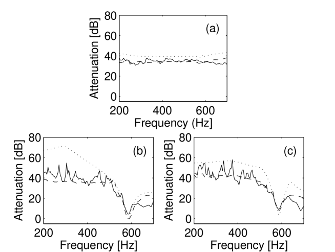
Figure 13:

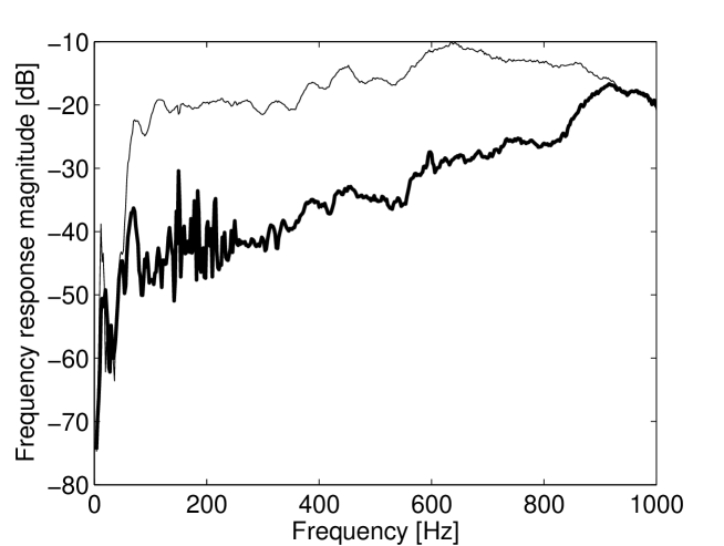
Figure 14:

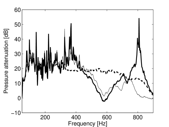
Figure 15:

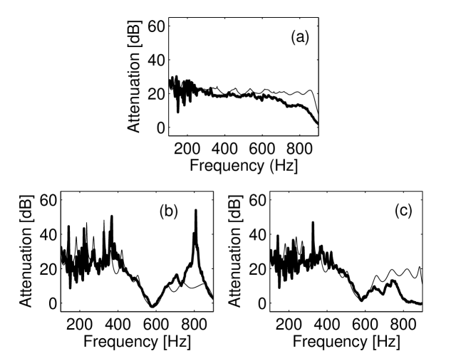
Figure 16:

References

- [1] D.R. Begault, 3-D Sound for Virtual Reality and Multimedia (AP Professional, Boston, 1994).
- [2] M.A. Gerzon, Ambisonics in Multichannel Broadcasting and Video Journal of the Audio Engineering Society 33 (1985) 859-871.
- [3] A.J. Berkhout, D. de Vries and P. Vogel, Acoustic Control by Wave Field Synthesis, Journal of the Acoustical Society of America 93 (1993) 2764–2778.
- [4] A. Dancer and P. Naz, Sonic Boom: ISL studies from the 60’s to the 70’s, in Proceedings of the Joint Congress CFA/DAGA’04 (2004), on CD-ROM (2 pages).
- [5] F. Coulouvrat, Le Bang Sonique Pour la Science 250 (1998) 24–29 (in French).
- [6] E. Corteel, U. Horbach, and R.S Pellegrini, Multichannel Inverse Filtering of Multiexciter Distributed Mode Loudspeakers for Wave Field Synthesis, in Proceedings of the 112th AES Convention (2002), on CD-ROM.
- [7] S. Spors, A. Kuntz, and R. Rabenstein, An Approach to Listening Room Compensation with Wave Field Synthesis, in Proceedings of the AES 24th International Conference (2003) 70–82.
- [8] O. Kirkeby and P.A. Nelson, Reproduction of Plane Wave Soundfields, Journal of the Acoustical Society of America 94 (1993) 2992–3000.
- [9] O. Kirkeby, P.A. Nelson, F. Orduna-Bustamante, and H. Hamada, Local Sound Field Reproduction Using Digital Signal Processing Journal of the Acoustical Society of America 100 (1996) 1584–1593.
- [10] P.A. Nelson, Active Control of Acoustic Fields and the Reproduction of Sound, Journal of Sound and Vibration 177 (1994) 447–477.
- [11] Y. Kahana, P.A. Nelson, O. Kirkeby and H. Hamada, A Multiple Microphone Recording Technique for the Generation of Virtual Acoustic Images, Journal of the Acoustical Society of America 105 (1999) 1503–1516.
- [12] J. Bauck and D.H. Cooper, Generalized Transaural Stereo and Applications, Journal of the Audio Engineering Society 44 (1996) 683–705.
- [13] O. Kirkeby, P.A. Nelson and H. Hamada, Local Sound Field Reproduction Using Two Closely Spaced Loudspeakers, Journal of the Acoustical Society of America 104 (1998) 1973–1981.
- [14] J.W. Choi and Y.H. Kim, Manipulation of Sound Intensity Within a Selected Region Using Multiple Sources, Journal of the Acoustical Society of America 116 (2004) 843–852.
- [15] S. Ise, A Principle of Sound Field Control Based on the Kirchhoff-Helmholtz Integral Equation and the Theory of Inverse Systems, ACUSTICA - Acta Acustica 85 (1999) 78–87.
- [16] S. Takane, Y. Suzuki and T. Sone, A New Method for Global Sound Field Reproduction Based on the Kirchhoff’s Integral Equation, ACUSTICA - Acta Acustica 85 (1999) 250–257.
- [17] T. Betlehem and T.D. Abhayapala, Theory and Design of Sound Field Reproduction in Reverberant Rooms, Journal of the Acoustical Society of America 117 (2005) 2100–2111.
- [18] P.A. Gauthier, A. Berry, and W. Woszczyk, Sound-field Reproduction In-room Using Optimal Control Techniques: Simulations in the Frequency Domain, Journal of the Acoustical Society of America 117 (2005) 662–678.
- [19] P.A. Nelson, F. Orduña-Bustamante and H. Hamada, Multichannel Signal Processing Techniques in the Reproduction of Sound, Journal of the Audio Engineering Society 44 (1996) 973–989.
- [20] M. Bruneau, Manuel d’acoustique fondamentale (Hermes, Paris, 1998) 288–289.
- [21] P.A. Nelson and S.J. Elliott, Active Control of Sound (Academic Press, London, 1992).
- [22] R.E. Kleinmann and G.F. Roach, Boundary Integral Equations for the Three-dimensional Helmholtz Equation, SIAM Review 16 (1974) 214–236.
- [23] A.N. Tikhonov and V.Y. Arsenin, Solutions of ill-posed problems (Winston & Sons, Washington D.C., 1977).
- [24] S.J. Elliott, Signal Processing for Active Control (Academic Press, London, 2001).
- [25] G. Mangiante, A. Roure and M. Winninger, Multiprocessor Controller for Active Noise and Vibration Control, in Proceedings of ACTIVE 1995 (1995), on CD-ROM (8 pages).
- [26] E. Leboucher, P. Micheau, A. Berry and A. L’Esp rance, A Stability Analysis of a Decentralized Adaptive Feedback Active Control System of Sinusoidal Sound in Free Space, Journal of the Acoustical Society of America 111 (2002) 189–199.
- [27] N. Epain, E. Friot and G. Rabau, Indoor Sonic Boom Reproduction Using ANC, in Proceedings of ACTIVE 2004 (2004), on CD-ROM (12 pages).