Qprop: A Schrödinger-solver for intense laser-atom interaction
Abstract
The Qprop package is presented. Qprop has been developed to study laser-atom interaction in the nonperturbative regime where nonlinear phenomena such as above-threshold ionization, high order harmonic generation, and dynamic stabilization are known to occur. In the nonrelativistic regime and within the single active electron approximation, these phenomena can be studied with Qprop in the most rigorous way by solving the time-dependent Schrödinger equation in three spatial dimensions. Because Qprop is optimized for the study of quantum systems that are spherically symmetric in their initial, unperturbed configuration, all wavefunctions are expanded in spherical harmonics. Time-propagation of the wavefunctions is performed using a split-operator approach. Photoelectron spectra are calculated employing a window-operator technique. Besides the solution of the time-dependent Schrödinger equation in single active electron approximation, Qprop allows to study many-electron systems via the solution of the time-dependent Kohn-Sham equations.
PROGRAM SUMMARY
Title of program: Qprop.
Catalogue number: To be assigned.
Program obtainable from: CPC Program Library, Queen’s University of Belfast, N. Ireland.
Computer on which program has been tested: PC Pentium IV, Athlon.
Operating system: Linux.
Program language used: C++.
Memory required to execute with typical data: Memory requirements depend on the number of propagated orbitals and on the size of the orbitals. For instance, time-propagation of a hydrogenic wavefunction in the perturbative regime requires about 64 KByte RAM (4 radial orbitals with 1000 grid points). Propagation in the strongly nonperturbative regime providing energy spectra up to high energies may need 60 radial orbitals, each with 30000 grid points, i.e., about 30 MByte. Examples are given in the article.
No. of bits in a word: Real and complex valued numbers of double precision are used.
Peripheral used: Disk for input–output, terminal for interaction with the user.
CPU time required to execute test data: Execution time depends on the size of the propagated orbitals and the number of time-steps.
Distribution format: Compressed tar archive.
Keywords: Time-dependent Schrödinger equation, split operator, Crank-Nicolson approximant, window-operator
Nature of the physical problem: Atoms put into the strong field of modern lasers display a wealth of novel phenomena that are not accessible to conventional perturbation theory where the external field is considered small as compared to inneratomic forces. Hence, the full ab initio solution of the time-dependent Schrödinger equation is desirable but in full dimensionality only feasible for no more than two (active) electrons. If many-electron effects come into play or effective ground state potentials are needed, (time-dependent) density functional theory may be employed. Qprop aims at providing tools for (i) the time-propagation of the wavefunction according to the time-dependent Schrödinger equation, (ii) the time-propagation of Kohn-Sham orbitals according to the time-dependent Kohn-Sham equations, and (iii) the energy-analysis of the final one-electron wavefunction (or the Kohn-Sham orbitals).
Method of solution: An expansion of the wavefunction in spherical harmonics leads to a coupled set of equations for the radial wavefunctions. These radial wavefunctions are propagated using a split-operator technique and the Crank-Nicolson approximation for the short-time propagator. The initial ground state is obtained via imaginary time-propagation for spherically symmetric (but otherwise arbitrary) effective potentials. Excited states can be obtained through the combination of imaginary time-propagation and orthogonalization. For the Kohn-Sham scheme a multipole expansion of the effective potential is employed. Wavefunctions can be analyzed using the window-operator technique, facilitating the calculation of electron spectra, either angular-resolved or integrated.
Restrictions onto the complexity of the problem: The coupling of the atom to the external field is treated in dipole approximation. The time-dependent Schrödinger solver is restricted to the treatment of a single active electron. As concerns the time-dependent density functional mode of Qprop, the Hartree-potential (accounting for the classical electron-electron repulsion) is expanded up to the quadrupole. Only the monopole term of the Krieger-Li-Iafrate exchange potential is currently implemented. As in any nontrivial optimization problem, convergence to the optimal many-electron state (i.e., the ground state) is not automatically guaranteed.
External routines/libraries used: The program uses the well established libraries blas, lapack, and f2c.
1 Introduction
Progress in the construction of lasers brings powerful sources of electromagnetic radiation into the laboratory. The frequency domain of modern lasers covers a wide range from the infrared to the ultraviolet. Laser intensities of W/cm2 and more are routinely achieved in many laboratories all over the world [1]. Such powerful light causes a number of strong-field phenomena like tunneling and above-threshold ionization, high order harmonic generation, nonsequential ionization, pronounced dynamic Stark-shifts, and the (not yet experimentally confirmed) dynamic stabilization [1, 2, 3, 4, 5, 6]. All these phenomena are not accessible through “conventional” perturbation theory where the external laser field is required to be small compared to the atomic binding force acting on the electron.
In the nonrelativistic regime (i.e., moderate charge states and moderate laser intensities Wcm-2), the solution of the time-dependent Schrödinger equation is the most rigorous nonperturbative approach to the problem of intense laser-atom interaction. Fortunately, most of the above mentioned phenomena (apart from nonsequential ionization) can be understood within a single active electron picture, making a numerical ab initio treatment possible at all. However, since an electron released by an intense laser may travel thousands of atomic units during the pulse, huge numerical grids in position space are needed. It was thus natural to investigate first low-dimensional model systems where the three electronic degrees of freedom were restricted to the laser polarization direction (see, e.g., [7, 8, 9, 10, 11]). Much qualitative insight was gained by these model studies while the quantitative agreement with experiment or full three-dimensional calculations is, in general, poor.
With continuously increasing computer power, two- and three-dimensional models of one and two-electron atoms were investigated. Two and three-dimensional studies of the single active electron dynamics in intense laser fields permit the use of elliptically polarized drivers, the calculation of angular distributions, and the investigation of the polarization properties of the light emitted into (high order) harmonics.
The methods used for the time-dependent propagation of the electronic wavefunction have been improved to lower the computational demand. Examples are variable time- and space stepping [12, 15], advanced finite difference approximations [13, 14], advanced interpolation methods like Gauss-Legendre or B-Spline interpolation [15, 16], higher-order time propagators [17, 18], or matrix iterative methods [19].
There exist alternative methods, which avoid the propagation of the time-dependent wave function on a numerical grid representing real position space. Instead, the -method [20], Floquet theory [21, 22], and complex scaling [23, 24, 22] make use of extended Hilbert spaces, (approximate) time-periodicity, or complex continuation of position space, respectively.
Codes propagating two-electron wavefunctions in their full dimensionality are currently at the limit of feasibility [13, 24, 25]. It is unlikely that more complex systems will be treated on an equal footing because of the exploding computational demand. Even if the final, high-dimensional, multi-electron wavefunction were available, its analysis would pose new problems. In other words, the brute-force approach to multi-electron atoms in intense laser fields is a dead end [26].
It is the Nobel-prize winning density-functional theory (DFT) that provides a genuine resort for quantum mechanics to treat many-electron systems as ab initio as possible. The central theorem of DFT, the Hohenberg-Kohn theorem, states that quantum mechanics may be based on the electron density alone. The density remains a three-dimensional quantity, independently of the number of particles in the system. As a consequence, density-functional theory does not suffer from the exponential explosion of computational demand, the so-called exponential wall [26]. In fact, DFT is now well-established in electronic structure calculations and quantum chemistry [26, 27, 28, 29, 30]. Most of the modern formulations of density-functional theory rely on the Kohn-Sham equations which provide a practicable computational scheme. Density-functional theory has been extended to the time-dependent domain [31, 32, 33, 34] and a number of algorithms for time-dependent Kohn-Sham-solvers have been published [35, 36, 37].
Two of the most interesting observable quantities are the spectrum of the radiation emitted by the atom and photoelectron spectra. The former can be easily calculated via the Fourier-transformation of the dipole acceleration while the latter is much more tricky. In principle, one should project the final wavefunction onto the (continuum) eigenstates of the unperturbed Hamiltonian. This is numerically very demanding, especially if the continuum eigenstates are analytically unknown. In contrast to the straightforward projection, implicit methods to calculate the photoelectron spectra can be of distinct advantage. In the Qprop code, a window-operator technique [38, 39] for the energy-analysis of the final wavefunction is employed, facilitating the calculation of total and angular-resolved photoelectron spectra without explicit determination of eigenstates.
The aim of this paper is to present a collection of routines that consistently realize three issues: (i) time-propagation of a wavefunction according to the time-dependent Schrödinger equation, (ii) time-propagation of Kohn-Sham orbitals according to the time-dependent Kohn-Sham equations, and (iii) the energy-analysis of the final one-electron wavefunction (or the Kohn-Sham orbitals). The actual algorithm for time propagation has been taken from [14], where it was introduced explicitly for the case of a linearly polarized laser field. In Qprop, we generalized the algorithm in two directions: (i) elliptic polarization, and (ii) effective many-electron potentials. For the exchange-part of the effective Kohn-Sham potential we use the expression suggested by Krieger, Li, and Iafrate [40]. The implementation of the window-operator routine for the spectral analysis of wavefunctions was inspired by the work of Schafer and Kulander [38].
Qprop does not posses a fixed input/output interface but rather is a library, functions of which realize the time-propagation and the analysis of the wavefunction. Hence, in order to profit from the program, the user should be familiar with the basics of the underlying theory and the algorithm. Both are presented in Secs. 2 and 3. Moreover, the five examples in Sec. 4 should ease the first steps. Additional examples, patches, updates, and further documentation are provided elsewhere [41]. The Qprop package has been successfully applied to a number of problems [42, 43, 44, 45, 46, 47, 48].
2 Theoretical background
2.1 Time-dependent first-principle equations
The nonrelativistic quantum dynamics of an electron is governed by the time-dependent Schrödinger equation, i.e., the electron wavefunction obeys222Atomic units () are used unless noted otherwise.
| (1) |
Here, spin degrees of freedom are neglected. The Hamiltonian may depend on time and in general reads
| (2) |
where and are vector and scalar potential, respectively. The operator is the canonical momentum while is the kinetic momentum so that is the kinetic energy. Extending the Schrödinger equation (1) to -electron systems is formally straightforward, leading to a -electron wavefunction in a -dimensional Hilbert space (spin neglected). In practice, however, current super computers are hardly capable of treating two-electron atoms in full dimensionality exposed to strong laser fields [25], let alone systems with more than two electrons.
Time-dependent density-functional theory (TDDFT) offers to reduce the numerical effort dramatically [31, 32, 33, 34]. The basic quantity of density-functional theory is the electron density , which is always a function of three space coordinates and time, independent of the number of particles . In practice, time-dependent density functional theory is formulated via the time-dependent Kohn-Sham equation
| (3) |
describing the evolution of the Kohn-Sham orbitals , the only physical significance of which is to build the electronic density according to
| (4) |
Kohn-Sham Hamiltonian and Schrödinger Hamiltonian differ only by an effective potential in the scalar potential . This effective potential depends on the Kohn-Sham orbitals themselves,
| (5) |
Thus, the Kohn-Sham equation corresponds to a set of nonlinear Schrödinger equations for the Kohn-Sham orbitals . From the numerical point of view the nonlinearity does not pose a serious problem. The important point is that (2) and (5) have the same structure so that the same propagation scheme can be used for both the Schrödinger wavefunction and the Kohn-Sham orbitals. In the following we shall present the propagation algorithm employed in the Qprop package.
2.2 Propagation algorithm
Short-time propagator
Equation (1), together with an initial wavefunction , governs the time evolution of for all times . Introducing the propagator
| (6) |
where denotes the time-ordering operator, one has
In most numerical approaches the time-propagation from the initial time to the final one is divided into small steps during which the possibly explicit time-dependence of the Hamiltonian and the time-ordering can be ignored so that the short-time propagator simplifies to
| (7) |
The finite-time propagation from to can be decomposed in a product of short-time propagators,
| (8) |
with .
Crank-Nicolson approximation for the short-time propagator
The short-time propagator (7) can be straightforwardly applied to a wavefunction only if the Hamiltonian is diagonal. In order to avoid diagonalization each time step the Crank-Nicolson333The last name of Phyllis Nicolson is often misspelled “Nicholson”. approximant is used [49]. The Crank-Nicolson approximation is easily motivated by the fact that the short-time propagation of half a timestep forward generates the same state as the propagation of half a timestep backward,
| (9) |
Expanding the exponent in the short-time propagator (7) in a Taylor series, the unitary Crank-Nicolson propagator (accurate to the third order in the time step )
| (10) |
is obtained. The actual implementation of the Crank-Nicolson propagator leads to an implicit algorithm. Because of the Hamiltonian in the denominator we cannot apply directly to a wavefunction (unless the Hamiltonian is diagonal). Hence, we go back to (9) and actually solve
| (11) |
for each time step. We observe that the Crank-Nicolson propagator requires the application of the Hamiltonian to the orbitals and . Further below we show how the wavefunction is expanded and discretized, leading to implicit matrix equations corresponding to (11).
Kohn-Sham Hamiltonian in the linearly polarized laser field
In this subsection we discuss the more general case of a Kohn-Sham Hamiltonian (5) keeping in mind that the Schrödinger Hamiltonian (2) is obtained by omitting the electron-electron interaction altogether. We write the Kohn-Sham Hamiltonian in the form
| (12) |
where, apart from the familiar kinetic energy term , the Hamiltonian contains the interaction with the electromagnetic field in dipole approximation, the central-field potential of the nucleus (or atomic core) , and the Kohn-Sham effective potential . In principle, the effective electron-electron interaction potential can be written as a functional of the total electronic density . In practice, it is approximated using the Kohn-Sham orbitals . Details on the implemented approximations will be presented below in Sec. 2.5. Here, we only assume that the radial multipole functions , in the expansion
| (13) |
are known. Terms , i.e., beyond the quadrupole, are neglected. Note that the expansion (13) holds for linearly polarized light only since the effective potential is assumed to remain azimuthally symmetric with respect to the polarization axis.
The interaction with the laser field in dipole approximation is usually established either in length or velocity gauge. Thus the interaction operator for linear polarization reads in general
| (14) |
where is the vector potential and is the electric field of the laser pulse. In the velocity gauge only the first two terms are present whereas in the length gauge only the third term is left. The purely time-dependent term is easily transformed away and, in fact, is by default not taken into account in Qprop. Depending on the problem, either length or velocity gauge may be advantageous. For instance, high-order above threshold ionization is treated in velocity gauge at lower computational cost than in length gauge [50]. The ionization rate of heavy ions, on the other hand, is more easily calculated using length gauge.
Radial–angular separation of the Hamiltonian
Atomic systems in their ground state manifest a prevailing spherical symmetry. Expanding the atomic orbitals in spherical harmonics ,
| (15) |
and inserting this expansion into (1) with the Kohn-Sham Hamiltonian (12) and the dipole interaction for linear polarization (14), a set of differential equations for the radial orbitals is obtained,
| (16) |
The latter equation shows that the radial orbitals for different magnetic quantum numbers are decoupled for a linearly polarized laser field in dipole approximation. Hence, the general expansion (15) can be reduced to
| (17) |
where the -th orbital possesses a single, well-defined magnetic quantum number . Consequently, only radial orbitals per Kohn-Sham orbital will be involved in the propagation for linear polarization, whereas radial orbitals are involved in the general expansion (15). The maximum orbital quantum number on the numerical grid is related to the number of absorbed photons and must be chosen sufficiently large. The spectral analysis explained in Sec. 2.6 below can be used to check whether was chosen properly (see also Sec. 4.4).
Breaking-down the Hamiltonian
Inserting the electron-electron interaction potential (13) into (16) and calculating the matrix elements with the spherical harmonics, (16) can be recast in the matrix form [14]
| (18) |
where denotes a column vector in -space,
| (19) |
and the matrices , , , , read
| (20) |
| (21) |
| (22) |
| (23) |
| (24) |
with
| (25) |
| (26) |
Note that is diagonal in -space, , , and couple an -component with while couples with .
The calculation of the spatial derivatives in and will be discussed below. Next, the matrix is split into a sum over mutually commuting matrices ,
| (27) |
| (28) |
Commutativity of the allows us to use the algebraic equation for the splitting of the corresponding propagator without introducing any additional errors,
| (29) |
Moreover, only two elements in the matrices are different from zero, making them effectively to matrices. Analogously, the Hamiltonians , , and can be decomposed in a sum of commuting terms as well.
Calculation of the spatial derivatives
The calculation of the spatial derivatives in and is implemented using improved finite difference expressions [14]. The radial orbitals are represented on an equidistant grid with grid spacing and grid points,
| (30) |
Implicit fourth order Simpson and Numerov expressions for the first and the second derivative are employed,
| (31) |
| (32) |
The finite difference operators and can be written as matrices, and , are given by
| (33) |
In order to ensure unitary time propagation, the matrix must be antihermitian. To that end the upper left and lower right corners of and are modified [14],
| (34) |
with .
In the case of the Coulomb potential , the second derivative of a radial -state orbital satisfies at the origin the relation
| (35) |
This fact can be taken into account by modifying the upper left elements in and [14],
| (36) |
Splitting of the time-propagator
Summarizing the previous sections, we write the Hamiltonian
| (37) |
where all terms can be written as a tensor product of operators acting either in “-space” or “-space,”
| (38) |
| (39) |
| (40) |
| (41) |
and are unity matrices, and , , and are matrices
| (42) |
The matrices and act on the th and ()th component of the wavefunction while the matrix acts on the th and ()th component.
The short-time propagator (7) with the Hamiltonian (37) is approximated up to third order in as the product
| (43) |
where each factor is approximated by the corresponding Crank-Nicolson expression (10).
Further details about the actual implementation of the propagation algorithm can be found in the documentation provided with the program and online at [41]. We only mention here that in Qprop the above described propagation procedure for linear polarization using expansion (17), as well as the more general algorithm for elliptical polarization using expansion (15) are implemented. The propagator in the latter case is even more complex than (43). It is used in the example in Sec. 4.5.
2.3 Imaginary time propagation
The time-dependent Schrödinger equation (1) determines the evolution of a quantum system in time, starting from an initial state . Often the initial state is the ground state of the unperturbed quantum system with
| (44) |
Ground states are analytically known only for a few specific potentials. In contrast, numerical approaches allow to find ground states for arbitrary potentials. They are often based on the fact that the total energy of the ground state is minimal. In Qprop the ground state can be determined using the ordinary propagation algorithm presented above in Sec. 2.2 with, however, the real time step replaced by an imaginary time step . Why this works may be seen as follows: Let an arbitrary wavefunction be expanded in eigenstates of the Hamiltonian . The wavefunction at later times then reads (without perturbations)
| (45) |
where are the eigenenergies corresponding to . Propagating one imaginary time step leads to
| (46) |
The factor is biggest for minimum , which means that during imaginary time propagation the corresponding state dies out slowest (if ) or explodes fastest (if ). The (renormalized) thus converges to the ground state .
The choice of the initial “guess” for the ground state wavefunction before imaginary time propagation is not critical but affects the time needed for convergence. The method even works with a random initial wavefunction, as it is illustrated in Sec. 4.1.
2.4 Imaginary absorbing potential
An obvious limitation of propagation in position space is the finite size of the numerical grid. Electron density approaching the boundaries—if treated without special care—will be reflected and may cause undesired, spurious effects. However, the electron density reaching the (sufficiently remote) boundary can be considered to contribute to ionization only but otherwise does not affect the dynamics of the atomic remainder. In order to avoid spurious effects it is desirable and, in fact, possible to formulate exact permeable boundary conditions. Unfortunately, such permeable boundary conditions are easily implemented in one-dimensional calculations only [52]. In three-dimensional calculations so-called “absorbing boundaries” [53], although not mathematically rigorous, proved to be most convenient and practicable. In Qprop the absorbing boundary is of the form with to be defined by the user. Clearly, should be a function that is close to zero in the main interaction region and increases up to a sufficiently high value at the grid boundary . A nonvanishing imaginary potential destroys unitary time propagation and thus leads to “dissipation” of the wavefunction. The decreasing norm may be used to evaluate the ionization probability (see example in Sec. 4.2).
2.5 Effective potentials
According to the Hohenberg-Kohn theorem (see, e.g., [26] and references therein), the electron density determines all observable quantities of a quantum systems, i.e., all observables are functionals of the density. Only a few of these functionals are known explicitly while many of them must be approximated in practice.
An electron density in an external potential yields the potential energy
| (47) |
while the exact kinetic energy as an explicit functional of the density is, in general, unknown.
Kohn and Sham (see, e.g., [26] and references therein) considered an auxiliary system of noninteracting electrons whose density coincides with the density of the real, interacting system. Because the auxiliary electrons do not interact with each other (but move in a common, effective potential), their Schrödinger equation separates, and the kinetic energy is simply the sum of one-particle kinetic energies,
| (48) |
The Kohn-Sham orbitals satisfy the Kohn-Sham equation
| (49) |
The only physical significance of the Kohn-Sham orbitals is to form the correct density
| (50) |
which, in turn, uniquely determines the potential , commonly split in the form
| (51) |
where denotes the same potential that is present in the interacting system’s Hamiltonian (e.g., ),
| (52) |
is the Hartree-potential accounting for the mutual repulsion of the electrons, and denotes the so-called exchange-correlation potential. The nuclear potential , although entirely independent of the electron density, can be formally written as the variational derivative of the external potential energy (47),
| (53) |
Analogously, the Hartree potential is the variational derivative of the electron-electron repulsion energy,
| (54) |
The exchange-correlation potential is split further into exchange and correlation potential, . In what follows, the correlation potential is neglected.
Approximations for time-dependent effective potentials
The time-independent Kohn-Sham equation (49) has its time-dependent counterpart, as already anticipated in Eqs. (1), (5), and (12). Analogous to the Hohenberg-Kohn theorem, the Runge-Gross theorem [31] asserts that also in the time-dependent case, the density determines all observable quantities.
In Qprop the time-dependent potentials of electron-electron repulsion and exchange are calculated adopting an adiabatic viewpoint, i.e., expressions known from stationary density functional theory are evaluated using the now time-dependent density . The effective potential (13) is written as a sum of Hartree and exchange potential,
| (55) |
The Hartree potential is expanded analogously to (13),
| (56) |
In the current version of Qprop the latter expansion is terminated (at latest) after the quadrupole term. The exchange potential is approximated using the expression proposed by Krieger, Li, and Iafrate (KLI) in [40]. Within the KLI approximation, going beyond the groundstate, monopole term turns out to be hard while in local density approximation it is simple to go up to the quadrupole term as well.
Hartree potential
The Hartree-potential (52) is calculated using the Kohn-Sham density (4) and the orbitals (17). Expanding in spherical harmonics, the following expressions for the Hartree multipoles in equation (56) are obtained,
| (57) |
| (58) |
| (59) |
where and are and , respectively. The auxiliary functions , , and read
| (60) |
| (61) |
| (62) |
The factor in these expressions stems from the spin degeneracy, i.e., we assume spin-unpolarized systems where each Kohn-Sham orbital is occupied by two electrons of opposite spin. The coefficients , , and are given by (25) and (26).
Krieger-Li-Iafrate approximation to the exchange potential
It is possible to derive an integral equation that implicitly defines the so-called optimized effective potential [54, 55, 56]. However, this integral equation is difficult to solve, and simpler expressions of comparable accuracy are needed in practice. Krieger, Li, and Iafrate (KLI) [40] simplified the full integral equation and obtained for the exchange potential
| (63) |
where denotes the spin variable of electrons,
| (64) |
is the spin density,
| (65) |
is the so-called Slater-potential, and
| (66) |
with the exact exchange energy
| (67) |
The integral equation (63) can be solved for by multiplying both sides with and integrating over space. Introducing the short-hand notation for the orbital average of an entity , the matrix equation
| (68) |
for the coefficients
| (69) |
is obtained. The matrix is given by
| (70) |
The term with the highest occupied spin orbital is excluded from the sums in (63) and (68) since it can be shown that [40]. After solving (68) for , all the quantities on the right hand side of (63) are determined, and the KLI potential can be evaluated.
Currently, only spin-unpolarized systems where , with the number of electrons in the system, and are tractable with Qprop. Orbital degeneracies are possible, so that no unnecessary overhead arises for Kohn-Sham orbitals that evolve identically in a laser field. For instance, the four orbitals with and behave identically in dipole approximation and thus can be subsumed under a single orbital of degeneracy .
Further computational details can be found in the documentation provided with the program and online [41]. In the current version of Qprop the KLI potential is restricted to the ground state monopole contribution . The latter is sufficient to determine state-of-the-art effective potentials for the ground state of spherically symmetric systems (or other systems in central field approximation). The ground state KLI potential may then be used for either frozen-core calculations or it may be re-calculated each time step as an approximation to the real TDDFT exchange potential. The latter approximation should be acceptable as long as most of the electrons stay inside the atom and the deviation from spherical symmetry remains small. The dipole contribution to the time-dependent KLI potential would be already very complicated due to the coupling of many angular momenta. Within simpler approaches (e.g., local density approximation) where the exchange potential is given explicitly as a functional of the density , an expansion up to the quadrupole is much simpler.
2.6 Spectral analysis: the window-operator technique
Qprop allows to calculate an initial state of interest and propagates this state in time. By the end of propagation—usually at the end of the laser pulse—the final state is obtained. It is useful to analyze its spectrum with respect to the Hamiltonian of the atomic system (without laser) whose eigenstates we denote by ,
| (71) |
In order to avoid the explicit calculation of all the eigenstates , a window-operator technique very similar to the one proposed in [38, 39] is employed. A window-operator of energy and of energy width is defined as
| (72) |
where is the integer order of the window-operator. The higher the order , the more rectangular is the window profile.
When acting on a state , the window-operator returns the energy component the scalar product of which gives a measure for the population of states that lie within the window of width , centered around the electron energy ,
| (73) |
Hence, for the modulus squared of the energy component equals . Finite energy width , on the other hand, allows to model realistic measurements with a finite energy resolution.
Since has the operator in the denominator, is actually calculated by solving the equation using the factorization
| (74) |
where the phases are uniformly distributed between and ,
| (75) |
In the current version of Qprop, the energy component is calculated for the fixed order for both the general (15) and the reduced expansion (17). is then obtained as an expansion in spherical harmonics with the radial energy components denoted by . The energy components in form of expansions over spherical harmonics allow to calculate differential probabilities of electron emission. The probability , differential in energy, reads
| (76) |
Useful information about the emission probability differential in energy and in angle is obtained by simply omitting the integration over the solid angle,
| (77) |
3 Program structure
The Qprop package is arranged as a library of classes whose objects represent orbitals, grids, and Hamiltonians. In order to use the library, an executable program has to be written. This program is usually short and may be regarded as an extended input-file which profits from all the powerful C++ features. Compared to a foolproofed approach where the user never makes direct contact with the actual data structures, our library-oriented approach requires more knowledge of the internal structures. On the other hand, once the user got acquainted with the important classes and functions, he or she may really benefit from the huge flexibility.
Content and functionality of the internal data structures will be considered in the following Sec. 3.1. The five examples in Sec. 4 are aimed at facilitating the first steps in the usage of Qprop.
3.1 Internal data structures
The classes fluid, wavefunction, grid, and hamop build the core of the Qprop library. Objects of classes fluid and wavefunction represent real valued and complex valued one-dimensional arrays, respectively.444The name “fluid” may appear strange. It is mainly for “historical” reasons since this class was originally developed for a fluid code that naturally deals with real valued arrays. The methods provided by these classes allow to initialize the corresponding arrays, to manipulate them, and to store (load) them to (from) files. From the physical point of view, objects of class wavefunction typically represent radial wavefunctions or sets of radial orbitals to be propagated. However, objects of class wavefunction may be used for any auxiliary quantity that can be represented by a complex vector. The heart of the Qprop library, namely the actual short-time propagation (43), is implemented as a member function of class wavefunction.
The entries of an object of class wavefunction are accessible through an object of class grid, which defines the number of spatial grid points, the number of angular momentum quantum numbers, the number of orbitals, the grid spacing, and whether expansion (15) or (17) is used. In other words, objects of class grid define the numerical grid on which the objects of class wavefunction are defined, e.g., the number of grid points in radial direction, the upper limit for the quantum numbers in the expansions (15) or (17), and the number of Kohn-Sham orbitals. The most important functions of class grid are collected in Tab. 1.
| Method | Arguments | Description and comments |
|---|---|---|
| set_dim | (long dim) | Defines type of expansion, i.e., either (15) dim=44 or (17) dim=34. |
| index | (long r, long l, long m, long n) | Calculates the index of a wavefunction (or orbital) entry; radial position r, angular momentum l, magnetic quantum number m, orbital no. n; n is irrelevant for dim=44 while m is irrelevant for dim=34 |
| set_delt | (double dr) | Defines |
| set_ngps | (long N_r, long L, long N_orb) | Defines , , and number of Kohn-Sham orbitals. |
| size | (void) | Returns size of grid object |
| r | (long rindex) | Calculates , given rindex |
| ngps_x | (void) | Returns number of radial gridpoints |
| ngps_y | (void) | Returns number of angular momenta |
| ngps_z | (void) | Returns number of orbitals |
Objects of class hamop collect a number of external potentials that set up the Hamiltonian. These potentials are to be defined by the user and are listed in Tab. 2.
| Function | Arguments | Description and comments |
|---|---|---|
| vecpot_x | (double t, int me) | -component of the vector potential (only relevant for dim=44, i.e., with Eq. (15)) |
| vecpot_y | (double t, int me) | -component of the vector potential (only relevant for dim=44, i.e., with Eq. (15)) |
| vecpot_z | (double t, int me) | -component of the vector potential (only relevant for dim=34, i.e., with Eq. (17)) |
| scalarpotx | (double x, y, z, t, int me) | Spherically symmetric potential in (16), x corresponds to , y and z are not needed |
| scalarpoty | (double x, y, z, t, int me) | since not used here |
| scalarpotz | (double x, y, z, t, int me) | since not used here |
| field | (double t, int me) | electric field in (16) |
| imagpot | (long xindex, yindex, zindex, | |
| double t, grid g) | imaginary potential from Sec. 2.4; xindex is the radial index for dim=34 or 44 while yindex and zindex are not relevant here |
Class wavefunction is clearly the most important part of the Qprop library. As already mentioned, it contains the methods to initialize, to load and to store the radial orbitals, to propagate them in time, to calculate the observable quantities and effective potentials. Table 3 shows some of the public methods to perform these tasks. Several methods are overloaded, i.e., they are distinguished by the different sets of arguments only. The meaning of most arguments is self-explanatory. Since many of the methods need to know in which order the radial orbitals are organized in the internal, one-dimensional array,555There are only one-dimensional arrays internally. the first argument often is of class grid. In order to control the verbosity of some complex methods, there is an integer iv argument at the end of the parameter list. Setting it to zero suppresses any output to the stdout stream.
| Method | Arguments | Description and comments |
|---|---|---|
| calculate_staticpot | (grid g, hamop hamil) | Calculates static part of total potential (scalarpotx + centrifugal potential + imagpot) using Hamiltonian hamil |
| calculate_Lambda | (grid g, fluid deg) | Calculates auxiliary quantity (60) |
| calculate_Theta | (grid g, fluid deg, fluid ms) | Calculates auxiliary quantity (61) |
| calculate_Xi | (grid g, fluid deg, fluid ms) | Calculates auxiliary quantity (62) |
| calculate_hartree_zero | (grid g, fluid Lambda) | Calculates monopole term (57) in expansion (56) |
| calculate_hartree_one | (grid g, wavefunction Theta) | Calculates dipole term (58) in expansion (56) |
| calculate_hartree_two | (grid g, wavefunction Xi) | Calculates quadrupole term (59) in expansion (56) |
| calculate_kli_zero |
(grid g, fluid Lambda, fluid ls, fluid ms, fluid deg,
int slateronly, int iv) |
Calculates groundstate KLI potential (63). Auxiliary array Lambda must be provided (see function calculate_Lambda() in this table). Flag slateronly=1 leaves only first summand on right hand side of (63) |
| dump_to_file_sh | (grid g, FILE file, int st, int iv) | Saves orbitals in file |
| energy | (double time, grid g, hamop hamil, int me, wavefunction staticpot, double charge) | Calculates kinetic energy plus potential energy due to static potential staticpot, e.g., bracket in equation (82) below |
| expect_z | (grid g) | Calculates for a single orbital. |
| expect_z | (grid g, fluid deg, const fluid ms) | Calculates for the entire set of Kohn-Sham orbitals. |
| init | (long size) | Various ways to initialize wavefunction objects (cf. examples in Sec. 4) |
| (grid g, int inittype, double w, fluid ls) | ||
| (grid g, FILE file, int ooi, int iv) | ||
| init_rlm | (grid g, int inittype, double w, fluid ls, fluid ms) | |
| propagate | (complex timestep, double time, grid g, hamop hamil, int me, wavefunction staticpot, int m, double nuclear_charge) | Propagates a wavefunction from time to time+timestep. hamil determines only external fields in this function. Potential of nucleus is supposed to be contained in staticpot (see calculate_staticpot() in this table). nuclear_charge is used to account for correction (36). There is an overloaded version for the propagation of several Kohn-Sham orbitals (cf. Sec. 4.3) |
| totalenergy_hartree | (grid g, fluid Lambda, fluid U_0) | Calculates Hartree energy (54) |
| totalenergy_exact_x | (grid g, fluid ells, fluid deg) | Calculates exchange energy (67) |
Objects of class fluid are basically real valued, one-dimensional arrays, i.e., the real counter parts of wavefunction objects. They are used to store effective potentials and auxiliary quantities that are not complex. For instance, calculate_hartree_zero in Tab. 3 returns an object of class fluid. Usage of the class is straightforward and can be understood from the examples in Sec. 4.
Apart from the classes wavefunction, grid, hamop and fluid, another class cmatrix and several functions are defined. Class cmatrix deals with matrix operations, some of which make use of the blas and lapack libraries. However, class cmatrix is currently used only inside member functions of class wavefunction so that there is no need to discuss its features in the present paper.
3.2 External libraries and source codes
Qprop needs the libraries blas, lapack, and f2c— all available free of charge [57, 58, 59]. Note that they are part of many Linux distributions. Apart from the libraries, Qprop profits from two programs to be cited: Clebsch-Gordan coefficients (needed for the KLI potential (63)) are calculated using the program ned by Arturo Sierra [60], and spherical harmonics (needed for the implementation of (77)) are calculated as in the Racah package [61].
3.3 Distribution and installation
The program is distributed as a single tarball qprop.tar.gz. The archive is organized in several subdirectories with source code, makefiles and README-files. Installation consists of extracting the tarball and creating links to the libraries blas, lapack, and f2c in the subdirectory lib/i386/. The top directory contains a makefile qprop/GNUmakefile.tmpl, which controls the compilation of the qprop library. The user will probably need to adjust the variable ROOT in this file. This variable points to the absolute location of the Qprop package.
 qprop/
       doc/
       lib/i386/
       obj/i386/
       src/
                base/
                circ/
                hydrogen/
                ionization/
                neon/
                winop/
Figure 1 shows the directory structure of the Qprop package. The basic source code is placed in the subdirectory src/base/. The code of several examples is placed in subdirectories in src/. Five examples are provided and discussed in Sec. 4.
The other directories contain extra documentation (in doc/), object files .o (in obj/i386/), and the library files (or links to) libqprop.a, libblas.a, liblapack.a, libf2c.a (in lib/i386/). The subdirectories with source code contain also the Makefiles so that the executable files can be compiled with the make utility. By default the executable is put in the same directory.
4 Test calculations
In order to facilitate a quick start, five examples for the application of the Qprop code are provided in the directories src/hydrogen/, src/ionization/, src/neon/, src/winop/, and src/circ/. The examples are chosen such that, on one hand they are not too run-time consuming while, on the other hand they cover in a non-trivial manner the key issues (i) imaginary time propagation, (ii) real time propagation, (iii) determination of an effective potential using DFT, (iv) calculation of electron spectra, and (v) circular polarization.
Each subdirectory in src/ contains the source code in the files with extension .cc and an appropriate Makefile to generate the executable program in the same directory. The output will be written to files in the subdirectories res.
4.1 Ground state via imaginary time propagation
The goal in this example is to calculate the nonrelativistic ground state of the hydrogen atom by means of imaginary time propagation. As explained in Sec. 2.3, imaginary time propagation is a powerful method to compute the ground state in any potential. The hydrogen atom was chosen because of its simplicity and the fact that the solution is analytically known. We start with an unbiased guess, that is, a random -orbital. The source code of the program hydrogen_im.cc is located in the subdirectory src/hydrogen/. In the following we discuss the few crucial points.
After standard directives concerning header files, the file potentials.cc is included.
// *** potentials, nuclear_charge, and laser pulse parameters
//     are declared in potentials.cc ***
#include<potentials.cc>
The file potentials.cc is a piece of code, which defines a few global variables and the potentials that make up the Hamiltonian. The idea is to put the code common to imaginary and real time propagation in an extra file, thus reducing liability to inconsistencies. The laser field is off (E_0=0.0) during imaginary time propagation.
Next, variables are declared and initialized. Let us consider the lines below the initialization of the object g of class grid:
// *** declare the grid ***
g.set_dim(34); // 44 elliptical polariz., 34 linear polariz.
g.set_ngps(1000,1,1);  // N_r, L, N
g.set_delt(0.2/nuclear_charge);  // delta r
g.set_offs(0,0,0);     // there is no offset in r, l, and N
Depending on the polarization of the laser light, the suitable expansion of the wavefunction in spherical harmonics is chosen, i.e., either (15) with all radial orbitals, suitable for any polarization in the -plane, or (17) for linear polarization along the -axis (where radial orbitals suffice). General and reduced expansion require different propagation procedures. Thus a propagation mode has to be specified using the set_dim() function. The next line g.set_ngps(1000,1,1) defines spatial grid points for each radial orbital , -quantum numbers (ranging from to ), and orbital. The hydrogen ground state requires only a single orbital of -symmetry so that is chosen. Since nuclear_charge is 1, follows, and the equidistant grid reaches up to au. There are no grid offsets for the two propagation modes 34 and 44 discussed in this paper so that the grid initialization is completed by g.set_offs(0,0,0).
The Hamiltonian hamilton of class hamop is initialized through the functions defined in potentials.cc:
// the Hamiltonian
hamilton.init(g,vecpot_x,vecpot_y,vecpot_z,scalarpotx,scalarpoty,scalarpotz,
                imagpot,field);

// this is the linear and constant part of the Hamiltonian
staticpot.init(g.size());
staticpot.calculate_staticpot(g,hamilton);
The time-independent part of the Hamiltonian is stored in staticpot (see calculate_staticpot in Tab. 3).
The radial wavefunction is stored in the object wf of class wavefunction. In this example there is only a single radial wavefunction because . The lines below initialize and normalize the wavefunction wf (dots “...” indicate lines of code that are omitted for the sake of clarity).
// *** wavefunction initialization ***
wf.init(g.size());
wf.init(g,iinitmode,1.0,ells);
wf.normalize(g);
...

wf.dump_to_file_sh(g,file_wf_ini,1)
Depending on the argument iinitmode of type int, the wavefunction may be initialized either randomly or with hydrogenic orbitals. The interested user may have a look at the corresponding init function in wavefunction.cc. In this example, the wavefunction is initialized randomly (iinitmode = 1) and written to file_wf_ini. (i.e., a file in the subdirectory src/hydrogen/res/). The file consists of two columns of numbers (real and imaginary part) and lines, i.e., only a single radial orbital in this example.
The array ells[] is used to assign the quantum number to the radial wavefunction . This information is solely needed by the initialization routine init when (see the more complex example 4.3 below).666If we choose and ells[0]=1 we obtain the state since only the radial wavefunction will be initialized with random numbers while . Note that there is no coupling between different quantum numbers during imaginary time propagation.
The actual propagation is a loop:
  // *** imaginary time propagation ***
  for (ts=0; ts<lno_of_ts; ts++)
  {
    time = time + imag(timestep);
    ...

    E_tot = real(wf.energy(0.0,g,hamilton,me,staticpot,nuclear_charge));
    ...

    wf.propagate(timestep, 0.0, g, hamilton, me, staticpot, 0, nuclear_charge);

    wf.normalize(g);
    ...

  }
Being inside the body of the loop, the short-time propagator is applied consecutively to the orbitals in wf with an imaginary time step g.delt_x()/4.0, i.e., here. The short-time propagation is handled by the wavefunction member function propagate() (cf. Tab. 3). Its first argument timestep is the pure imaginary time step. The second argument, i.e., the time, is irrelevant for the determination of the ground state and thus set to zero. Grid, Hamiltonian, process ID me, constant potential part staticpot, magnetic quantum number , and nuclear_charge (as defined in potentials.cc) follow as arguments.
In the loop body the total energy is calculated each imaginary time step so that one may keep track of the convergence of the total energy. After each propagation step the function is normalized because propagation in imaginary time is not unitary.
Imaginary propagation stops when a key is hit, i.e., when the user is satisfied with the convergence of the ground state energy, or at latest after lno_of_ts = 640000 time steps. After propagation, the orbital is stored in file_wf_fin in src/hydrogen/res/. The converged ground state energy on the numerical grid chosen above reads au.
The names of the files generated in src/hydrogen/res/ depend on the simulation parameters and read in the case discussed here
hydrogen_im-34-1000-2.00e-01.log
hydrogen_im_info-34-1000-2.00e-01.dat
hydrogen_im_obser-34-1000-2.00e-01.dat
hydrogen_im_wf_fin-34-1000-2.00e-01.dat
hydrogen_im_wf_ini-34-1000-2.00e-01.dat
The first file is a log-file containing all the important simulation parameters for inspection by the user. The second file is a xml-file from which other programs may conveniently read the simulation parameters. Observables are stored in the third file (time step and energy in two columns). Fourth and fifth file contain the wavefunction after and before the imaginary time propagation.
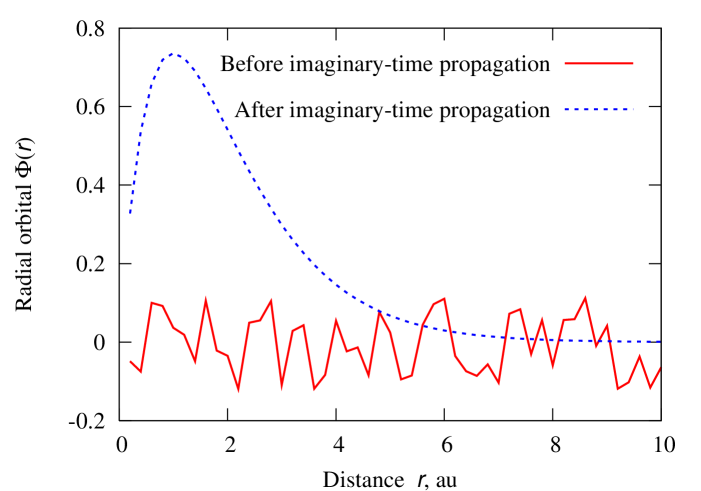
The radial wavefunctions before and after imaginary time propagation are shown in Fig. 2. The wavefunction after imaginary time propagation converged to the radial wavefunction .
The program hydrogen_re.cc in the same directory reads the wavefunction from file hydrogen_im_wf_fin-34-1000-2.00e-01.dat and propagates it in real time with the laser field switched on. The essential lines are provided with comments so that the code should be self-explanatory. Additional entities of interest such as the time-resolved ground state population, the expectation value in laser polarization direction , and the total norm on the grid are calculated inside the main propagation loop.
4.2 One, two, and three-photon ionization of hydrogen
The results presented in this example were obtained using the code in src/ionization. First, the hydrogen ground state is generated again using hydrogen_im.cc. Afterwards, the wavefunction is propagated in a -cycle -pulse ( with respect to the electric field)
| (78) |
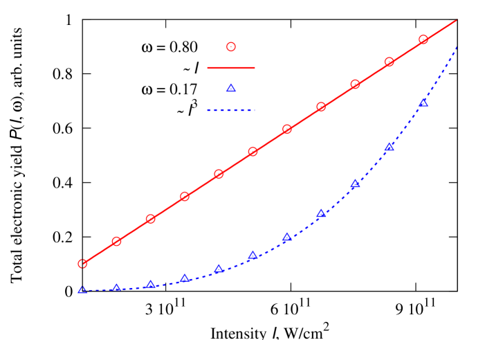
for different laser intensities between and Wcm-2 using ionization.cc. The vector potential corresponding to (78), i.e., , is implemented in potentials.cc. We want to focus on one and three-photon ionization. To that end we chose and , respectively.
It is well known that if the ponderomotive energy
| (79) |
i.e., the time-averaged quiver energy of a free electron in a laser pulse of amplitude , is much smaller than the ionization potential , ionization will be a perturbative process in the multiphoton regime, and perturbation theory in lowest nonvanishing order (LOPT) is sufficient.
The number of photons needed to overcome the ionization potential of the atom is given by
| (80) |
where is the energy of a photon and denotes the smallest integer . Thanks to the small ponderomotive energy the ac Stark shift can be omitted.
If the photon energy is smaller than the ionization potential, one-photon ionization is impossible because of energy conservation. On the other hand, , , photon ionization is possible but unlikely in the LOPT regime. The latter predicts that the ionization rate for a -photon process is proportional to the -th power of the light intensity (see, e.g., [5]), i.e.,
| (81) |
where the coefficient denotes the generalized cross section for -photon ionization. As long as the ionization probability is also proportional to . Figure 3 shows the numerical results obtained with ionization.cc in src/ionization, confirming the power-law behavior in the multiphoton LOPT regime.
4.3 Calculation of the neon ground state configuration
In this example, the total energy of the neon atom will be calculated within the Kohn-Sham formalism of density-functional theory. The theoretical background is presented above in Sec. 2.
In our nonrelativistic treatment, the total ground state energy of the neon atom can be calculated using only the three Kohn-Sham orbitals , , and , occupied by , , and “electrons”, respectively,
// *** declare the grid ***
nuclear_charge = 10.0;
g.set_dim(34); // only 34 (linear polariz.) works in Kohn-Sham mode
g.set_ngps(10000,2,3);  // we need 2 angular momenta and 3 orbitals here
g.set_delt(0.01);
g.set_offs(0,0,0);
The lines
  really_propagate[0] = 1; // orbital 0 is to be propagated (not frozen!)
  really_propagate[1] = 1; // orbital 1 is to be propagated (not frozen!)
  really_propagate[2] = 1; // orbital 2 is to be propagated (not frozen!)

  degener[0]          = 2; // two electrons in 1s shell
  degener[1]          = 2; // two electrons in 2s shell
  degener[2]          = 6; // six electrons in 2p subshell

  ms[0]               = 0; // m quantum number of orbital 0
  ms[1]               = 0; // m quantum number of orbital 1
  ms[2]               = 0; // whether one puts 0,1, or -1 here
                           // does not matter for the ground state

  ells[0]             = 0; // l quantum number of orbital 0
  ells[1]             = 0; // l quantum number of orbital 1
  ells[2]             = 1; // l quantum number of orbital 2
are self explanatory. They assign and quantum numbers, degeneracies (i.e., occupation numbers), and the information whether orbital no. should be really propagated (really_propagate[]=1) or considered frozen (really_propagate[]=0).
As compared to the simpler case of atomic hydrogen in Sec. 4.1 the overloaded Kohn-Sham version of propagate() requires the radial functions , , and from the multipole expansion (13) as arguments:
Lambdavector = wf.calculate_Lambda(g,degener);
U_H0 = wf.calculate_hartree_zero(g,Lambdavector);
U_x0 = wf.calculate_kli_zero(g,Lambdavector,ells,ms,
                             degener,islateronly,0);
V_ee_0 = U_H0 + U_x0;


wf.propagate(timestep, 0.0, g, hamilton, me, staticpot,
             V_ee_0, V_ee_1, V_ee_2, ms, nuclear_charge, really_propagate);

wf.normalize(g,ms);
Because all shells in ground state neon are closed, the electron density distribution is spherical, and so is the effective potential. Thus the monopole term of the effective potential is sufficient. The same holds for open-shell systems in the commonly applied central field approximation. The function normalize(g,ms) performs a Gram-Schmidt orthonormalization of the Kohn-Sham orbitals. Exchange potential (in KLI approximation) and Hartree potential are calculated using calculate_kli_zero() and calculate_hartree_zero(), respectively.
Next, a few characteristic energies are calculated and written to the file file_obser_imag
//
// calculate energies
//
orb_energs = wf.orbital_energies(0.0, g, hamilton,me,
                                 staticpot, nuclear_charge);
orb_hartreesandexchange = wf.orbital_hartrees(0.0,g,me,U_H0+U_x0);
E_sp = wf.totalenergy_single_part(g,orb_energs, degener);
hartree_energy = wf.totalenergy_hartree(g,Lambdavector,U_H0);
x_energy=wf.totalenergy_exact_x(g,ells,degener);
E_tot = real(E_sp + hartree_energy + x_energy);
//
// output to observables file
//
fprintf(file_obser_imag,"%i %15.10le %15.10le %15.10le %15.10le ",
        ts,E_tot,E_sp,real(hartree_energy),real(x_energy));
for (i=0;i<g.ngps_z();i++)  // loop over KS orbitals
               fprintf(file_obser_imag,
               "%15.10le ",real(orb_energs[i]+orb_hartreesandexchange[i]));
Here, we defined the orbital energy of Kohn-Sham orbital as
| (82) |
The result is stored in the array orb_energs. The single-particle energy is defined as
| (83) |
i.e., the orbital energies , weighted by the occupation numbers . The total energy is then given by
| (84) |
with according (54) and according (67). The orbital energies in (49) are given by
| (85) |
where
| (86) |
denotes the orbital contribution due to the electron-electron interaction. In the code above, is stored in the array orb_hartreesandexchange. The sum of orb_energs[] and orb_hartreesandexchange[] gives , which is written to file file_obser_imag as well. Note that owing to the nonlinearity of the Kohn-Sham equation .
| , au | exact KLI | LDA for Ne in [63] | ||||
|---|---|---|---|---|---|---|
| , au | ||||||
| , au | ||||||
| , au | ||||||
| , au | ||||||
| , au | ||||||
| , au | 12.099 | |||||
| , au | 128.5448 |
The numerical results for different grid spacings are collected in Tab. 4. Very good agreement with the exact KLI values is obtained. Of particular interest is the orbital energy of the valence electron, i.e., . Imagine we want to use the effective potential for a single active electron calculation where only the valence electron is propagated while all others are kept “frozen”. Such an approach will only lead to quantitative correct answers if the modulus of the orbital energy is close to the first ionization potential (i.e., if Koopmans’ theorem [64] is satisfied). The ionization potential of neon is showing that KLI yields an enormous improvement compared to the simpler local density approximation (LDA) which is % off.
A few remarks are advisable at that point.
-
1.
In the current version of Qprop the KLI potential is implemented for the search of the ground state configuration only. Unfortunately, the multipole expansion of the KLI expansion is utterly complicated if the Kohn-Sham orbitals loose their well-defined quantum number (as it is the case when the laser field is switched on). For more details see the extra documentation in doc or online [41]. The Hartree potential, on the other hand, can be evaluated using the time-dependent, perturbed Kohn-Sham orbitals up to the quadrupole.
-
2.
As in any nontrivial optimization problem, it is not given for granted that the Gram-Schmidt orthonormalization during imaginary time propagation in the Kohn-Sham mode converges to the correct ground state configuration. The better are the initial guesses for the orbitals, the higher is the chance to find the true ground state. For the case of neon with only a few orbitals this is not a critical issue. We found out that for heavier atoms it is a good strategy to “build up” the electron configuration step by step, i.e., starting with an ion and adding one electron after the other. In that way we successfully generated the ground state configuration of xenon.
-
3.
With a bad initial guess the orbital energies may cross during imaginary time propagation. However, for a proper KLI potential it is important that the last orbital (i.e., the orbital with the highest index ) remains the outermost one during imaginary time propagation, since it is this orbital that is excluded from the sum in (63). Moreover, the sequence of orbitals must remain consistent with their degeneracies.
-
4.
It is instructive (and a good test) to choose instead of the three orbitals above five orbitals , , , , , all occupied by electrons. The results in Tab. 4 are not affected, of course.
4.4 Energy analysis of the final wavefunction
Besides the actual time propagation, the Qprop package provides a tool to evaluate energy spectra and angular distributions of the photoelectrons. The spectral analysis of the final wavefunction is performed using the window-operator approach introduced in Sec. 2.6. Here, we present an implementation of it called Winop.
The program winop.cc is located in the subdirectory src/winop. It computes the probability distributions (76) and (77) from a one-electron wavefunction given in form of either the expansion (15) or expansion (17).
First, the energy range and spectral resolution is defined:
//
//  set a few essential parameters for the calculation of the spectra
//
lnoofwfoutput       = 1;      // 0 -- initial state, 1 -- final state.
no_energ            = 2750;   // number of energy bins
gamma               = 1.0e-4; // half width of the window operator (72)
energy_init         = -0.55;  // first energy; last energy then is
                              // energy_init + (no_energ-1)*2*gamma

// define for how many angles (77) should be evaluated
no_theta            = 1; // no_theta angles between 0 and (1-1/no_theta)*pi
no_phi              = 1; // no_phi angles between 0 and (1-1/no_phi)*2*pi
The variable lnoofwfoutput specifies which of the stored wavefunctions should be considered for the calculation of the spectrum. This is important if several wavefunctions (or orbitals) are saved in the same file. In src/hydrogen/hydrogen_re.cc, for instance, the wavefunction is saved two times: before the propagation loop and after so that lnoofwfoutput can be 0 (for an analysis of the initial wavefunction) or 1 (for the analysis of the final wavefunction).
The next three parameters define the spectral range and resolution. The latter is governed by the parameter of the window-operator (72): the smaller it is the higher is the spectral resolution. The variables no_theta and no_phi specify the number of angles for which the directional spectra (77) are evaluated.
In order to ensure that the spectra are really calculated with respect to the proper Hamiltonian, the same potentials.cc-file should be used for both the wavefunction propagation and the spectral analysis. For the latter only the unperturbed, spherically symmetric Hamiltonian is taken into account.
The grid associated with the wavefunction to be loaded is determined from the info-file generated by the propagation program (e.g., hydrogen_re.cc in src/hydrogen) and stored in g_load. It is sometimes advisable to calculate the spectra on a grid that is larger than the grid on which the wavefunction was obtained because the energy resolution in the continuum increases when the grid radius is increased. In fact, our numerical grid is a spherical box whose discrete energy levels lie the closer together the bigger the radius is chosen. Since the level spacing increases with increasing energy, high resolution at high energies is only obtained for sufficiently large grid radii. Grid g is used for the analysis. The loaded wavefunction is then regridded from g_load to g.
The core of winop.cc is a loop over the energy bins centered at . Inside the loop, the function
 winop_fullchi( fullchi, result_lsub, &result_tot, energ, gamma,
                staticpot, V_ee_0, nuclear_charge, g, wf, iv);
calculates the state for order and gives it back as an object of class wavefunction, named fullchi. The latter is needed to evaluate (76) and (77). The partial results
| (87) |
are of interest because they reflect selection rules related to angular momentum. They are returned via the array result_lsub. Moreover, the partial spectra (87) may be used to check the convergence of the wavefunction propagation with respect to the number of angular momenta : if the partial contribution for is sizeable, should be increased.
The output of winop.cc to file file_res in the case of the restricted expansion (linear polarization) (17) is organized as follows:
| column 1 | columns 2 to | column | columns to no_phi*no_theta |
|---|---|---|---|
| Energy | part. spectra Eq. (87) | total Eq. (76) | angular resolved Eq. (77) |
In the last no_phi*no_theta columns the results are stored in the form
with no_theta and no_phi.
In the case of the general expansion (15) we have additional output for the various quantum numbers:
| column 1 | columns 2 to | column | columns to no_phi*no_theta |
|---|---|---|---|
| Energy | part. spectra Eq. (87) | total Eq. (76) | angular resolved Eq. (77) |
Columns 2 to contain the in the form
i.e., is the faster running index.
The actual winop.cc example-file the user finds in the src/winop-directory reads the final wavefunction generated by the example for circular polarization in the following Sec. 4.5. However, the user may try to adapt the winop.cc-file in order to analyze a final wavefunction generated by ionization.cc described in Sec. 4.2.
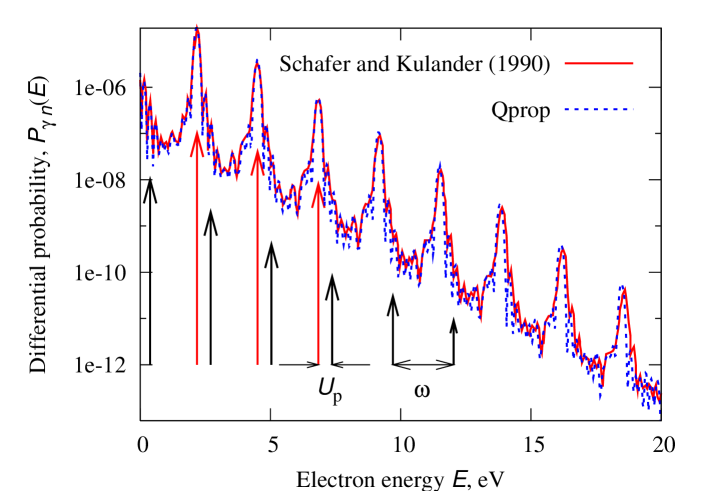
As a test we reproduced the photoelectron spectrum obtained by Schafer and Kulander in [38]. The laser parameters were chosen as specified in [38]. They are explicitly given in the caption of Fig. 4. The photon energy eV corresponds to six-photon ionization in lowest order. Since we have to allow for multiphoton absorption with each photon increasing the angular quantum number by one, was set to . The fastest electrons to be resolved in the spectrum must not reach the absorbing boundary within the simulation time. To be safe, 40000 grid points in radial direction and were chosen.
After having generated the final wavefunction with Qprop, Winop was used to calculate the spectrum shown in Fig. 4. One clearly identifies eight above-threshold ionization peaks. The peaks are located at
and separated by . The -shift away from the “naively” expected position at is due to the ac Stark-effect. The integer is the smallest integer that yields .
4.5 Rabi-flopping in a circularly polarized laser field
In the last example we consider a hydrogen atom, driven resonantly by a circularly polarized laser field in dipole approximation,
| (88) |
The field vector rotates clockwise in the -plane. The laser frequency is chosen to be resonant with the -transition,
Owing to the resonant driving a two-level approximation is adequate for not too high field amplitudes , i.e.,
| (89) |
Here we assume that the atom starts in the ground state, and we make use of the fact that the level with will be predominantly populated (as will be justified below). The time evolution of the two populations and is then governed by the differential equations
| (90) | |||||
| (91) |
where
| (92) |
As a consequence, the ground state population evolves according
| (93) |
where is the so-called Rabi frequency (see any text book on quantum optics, e.g., [65]). In our case one has
| (94) |
The example code can be found in the subdirectory src/circ. Since we are dealing with circular polarization we need to employ the general expansion (15) and therefore set g.set_dim(44). The program circ_im.cc generates the hydrogen ground state on a numerical grid with , , and . The ground state wavefunction (stored in ./res/circ_im_wf_fin-44-1000-1.50e-01.dat) and the corresponding info file (stored in circ_im_info-44-1000-1.50e-01.dat) are read by the program circ_re.cc, which performs the actual time propagation.
The propagation algorithm for elliptical polarization using the wavefunction expansion (15) is significantly more involved than the method for linear polarization explained in Sec. 2.2. A detailed description can be found online at [41] and in the directory doc. Here we only note that in propagation mode the vector potential must be of the form
| (95) |
so that the Hamiltonian (with the purely time-dependent term transformed away) reads
| (96) |
where
| (97) |
The vector potential components and are defined in potentials.cc. In order to match (88) they are chosen as
| (98) |
Real time propagation is performed for (corresponding to W/cm2) on a numerical grid with , , and . The expected Rabi-frequency (94) is . Fig. 5 shows that the temporal behavior of the ground state population (i.e., the third column in the output file ./res/circ_re_obser-0.375000-44-1000-1.50e-01.dat) is in excellent agreement with Eq. (93).
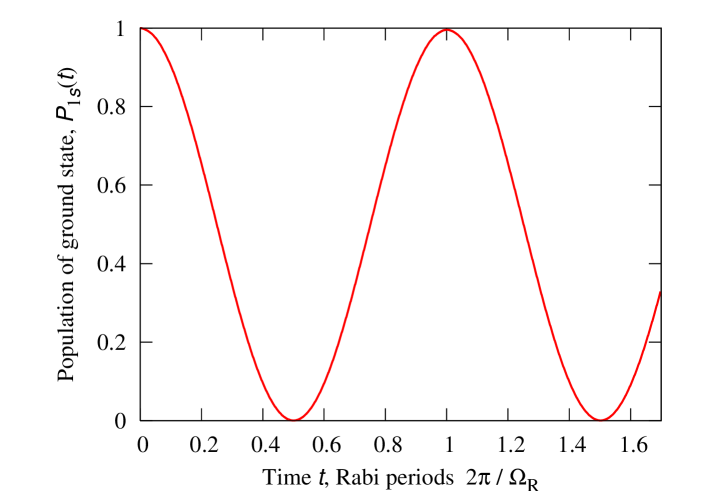 |
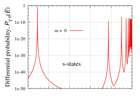
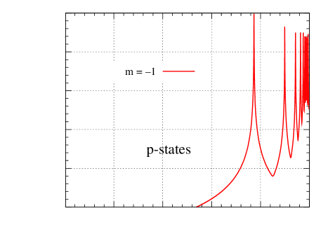
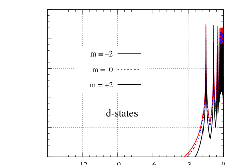
Figure 6 shows the result of a spectral analysis using the program winop_circ.cc777This file should be copied to winop.cc before using make for compilation. in src/winop, which reads the final wave function stored in src/circ/res/circ_re_wf-0.375000-44-1000-1.50e-01.dat and the corresponding info file. Moreover, potentials.cc in src/circ is included for the proper definition of the unperturbed Hamiltonian. The spectra are calculated in the energy range with a resolution .
|
|

|
|
On the logarithmic scale down to and beyond in Fig. 6 many more states than just the and the are populated. However, looking up the populations of the -levels at in the file ./res/res-0.375000-44-1000-4-2.000e-04-1.000e-04.dat one infers that the next “important” state (the ) is already a factor less populated than the . Hence, the two-level approximation is very well applicable at W/cm2.
By virtue of the partial spectra in ./res/res-0.375000-44-1000-4-2.000e-04-1.000e-04.dat it is also observed that the population of all states , , , , , remain exactly zero. This is because all couplings generated by the Hamiltonian (96) (with a vector potential (97)) require and . As long as one starts with a well-defined state of the unperturbed system one could remove all the strictly unpopulated states in the expansion (15), thus saving a considerable amount of run-time. In cases where, for instance, the initial state is the ground state one could replace the general expansion (15) by
where runs in steps of , i.e., . However, we did not implement this in the present version of Qprop in order to allow also for the propagation of superpositions of states with different s.
It is interesting to increase the laser intensity so that more and more states—including the continuum—become involved, and the two-level approximation breaks down. Note that for obtaining converged results both and must be increased appropriately. It is known that at higher laser intensity the lowest-order photoelectron peak at splits into two, separated by the Rabi frequency [66]. The interested reader may try to reproduce this result using Qprop.
4.6 Other tests
Besides Kohn-Sham orbital energies and the comparison in Fig. 4, additional tests of the Qprop package have been performed. Ionization rates were determined from the time-dependent norm on the numerical grid and compared with the highly precise ionization rates obtained with the help of the Floquet code [21]. Excellent agreement is obtained for sufficiently small and , and sufficiently large grid. The grid size is either determined by the excursion of the electrons in the laser field or the distance travelled by the fastest electrons that should be resolved in the final photoelectron spectra. If it is not necessary to resolve electrons beyond a certain threshold energy they may well be absorbed by the imaginary potential without spoiling the observables of interest. In any case, checking the results for convergence with respect to grid size, , and is a must.
The code was further tested by propagating a free Gaussian wave packet in a laser field—a problem that can be solved analytically. If, with increasing laser amplitude (i.e., increasing excursion) both the number of grid points in radial direction and the maximum -quantum number were increased appropriately, excellent agreement was obtained.
Our simulations of high order harmonic generation in many-electron atoms indicate that the truncation of the Hartree potential expansion after the quadrupole is safe: the spectra hardly change when the quadrupole term is omitted. Even the monopole alone is sufficient for a wide range of laser parameters.
5 Summary and Outlook
The Qprop package has been introduced. The purpose of the package is to study atoms or other (initially) spherical systems in strong laser fields. Qprop allows to investigate a great variety of nonperturbative phenomena including above-threshold ionization, high-order harmonic generation, and stabilization. The full time propagation of nonrelativistic, one-electron wavefunctions is realized. Effective potentials incorporating electron-electron repulsion and exchange can be taken into account. Further development will be aimed at removing the following restrictions:
The external field is currently treated in dipole approximation only, i.e., is approximated by . Going beyond the dipole approximation by taking into account the next order, , allows to study new phenomena related to the -electron drift in -direction. The azimuthal symmetry is broken then so that (15) has to be employed.
Many-electron systems can be currently treated only on a Kohn-Sham level using either the local density approximation or KLI. Although ab initio in principle, many important observables cannot be calculated in practice because their functional dependences on the Kohn-Sham orbitals are unknown. If, on the other hand, the full, generally correlated, many-electron wavefunction (or a reasonable approximation to it) is available, the computation of observables is straightforward. However, already the time propagation of a two-electron wavefunction is a demanding task [13, 25] as soon as the continuum becomes involved. For few-electron systems, the time-dependent multi-configurational Hartree-Fock method or related approaches are worth being investigated. Our current activities show that the implementation of such kind of schemes benefits heavily from the routines provided by Qprop.
Acknowledgement
This work was supported by the Deutsche Forschungsgemeinschaft.
References
- [1] P. Agostini and L. F. DiMauro, Rep. Prog. Phys. 67 (2004) 813.
- [2] W. Becker, F. Grasbon, R. Kopold, D.B. Milošević, G.G. Paulus, and H. Walther, in Adv. At. Mol. Opt. Phys. 48 (2002) 35.
- [3] C.J. Joachain, M. Dörr and N.J. Kylstra, in Adv. At. Mol. Opt. Phys. 42 (2000) 225.
- [4] Th. Brabec and F. Krausz, Rev. Mod. Phys. 72 (2000) 545.
- [5] N. B. Delone and V. P. Krainov, Multiphoton processes in atoms (Springer, Berlin, 1999).
- [6] M. Protopapas, C.H. Keitel, and P.L. Knight, Rep. Prog. Phys. 60 (1997) 389.
- [7] Q. Su and J. H. Eberly, Phys. Rev. A 44 (1991) 5997.
- [8] Ue-Li Pen and T. F. Jiang, Phys. Rev. A 46 (1992) 4297.
- [9] Qun Chen and Ira B. Bernstein, Phys. Rev. A 47 (1993) 4099.
- [10] R. Grobe and J. H. Eberly, Phys. Rev. A 48 (1993) 4664.
- [11] M. S. Pindzola, P. Gavras, and T. W. Gorczyca, Phys. Rev. A 51 (1995) 3999.
- [12] Charles Cerjan and Ronnie Kosloff, interactions Phys. Rev. A 47 (1993) 1852.
- [13] Edward S. Smyth, Jonathan S. Parker and K. T. Taylor, Comp. Phys. Comm. 114 (1998) 1.
- [14] H. G. Muller, Laser Physics 9 (1999) 138.
- [15] Xiao-Min Tong, Shih.-I. Chu, Chem. Phys. 217 (1997) 119.
- [16] H. Bachau, E. Cormier, P. Decleva, J. E. Hansen and F. Martín, Rep. Prog. Phys. 64 (2001) 1815.
- [17] I. V. Puzynin, A. V. Selin and S. I. Vinitsky, Comp. Phys. Comm. 126 (2000) 158.
- [18] Charles Cerjan and K. C. Kulander, Comp. Phys. Comm. 63 (1991) 529.
- [19] M. Nurhuda and F.H.M. Faisal, Phys. Rev. A 60 (1999) 3125.
- [20] Uri Peskin and Nimrod Moiseyev, J. Chem. Phys. 99 (1993) 4590.
- [21] R.M. Potvliege, Comp. Phys. Comm. 114 (1998) 42.
- [22] Shih-I Chu and Dimitry A. Telnov, Phys. Rep. 390 (2004) 1.
- [23] W. Reinhardt, Annu. Rev. Phys. Chem. 33 (1978) 223.
- [24] Armin Scrinzi and Bernard Piraux, Phys. Rev. A 58 (1998) 1310.
- [25] K. J. Meharg, J. S. Parker and K. T. Taylor, J. Phys. B 38 (2005) 237.
- [26] W. Kohn, Rev. Mod. Phys. 71 (1999) 1253.
- [27] R.M. Dreizler and E.K.U. Gross, Density Functional Theory (Springer, Berlin, 1990).
- [28] R.G. Parr and W. Yang, Density-Functional Theory of Atoms and Molecules (Oxford University Press, Oxford, 1989).
- [29] D. Joubert, Density Functionals: Theory and Applications (Springer, Berlin, 1998).
- [30] C. Fiolhais, F. Nogueira, M. Marques (Eds.), A Primer in Density Functional Theory (Springer, Heidelberg, 2003).
- [31] Erich Runge and E.K.U. Gross, Phys. Rev. Lett. 52 (1984) 997.
- [32] K. Burke and E.K.U. Gross, in [29] p. 116.
- [33] C.A. Ullrich, S. Erhard, and E.K.U. Gross, in Super Intense Laser Atom Physics IV, H.G. Muller and M.V. Fedorov, (Eds.) (Kluwer, 1996) p. 267.
- [34] Miguel A.L. Marques and E.K.U. Gross, in [30] p. 144.
- [35] Miguel A. L. Marques, Alberto Castro, George F. Bertsch and Angel Rubio, Comp. Phys. Comm. 151 (2003) 60.
- [36] W. Russel Burdick, Yousef Saad, Leeor Kronik, Igor Vasiliev, Manish Jain and James R. Chelikowsky, Comp. Phys. Comm. 156 (2003) 22.
- [37] Xiao-Min Tong, Shih.-I. Chu, Phys. Rev. A 57 (1998) 452.
- [38] K. J. Schafer and K. C. Kulander, Phys. Rev. A 42 (1990) 5794.
- [39] K. J. Schafer, Comp. Phys. Comm. 63 (1991) 427.
- [40] J. B. Krieger, Yan Li and G. J. Iafrate, Phys. Rev. A 45 (1992) 101.
- [41] http://www.qprop.de
- [42] D. Bauer, D.B. Milošević, and W. Becker, J. Mod. Opt. (in press)
- [43] D.B. Milošević, D. Bauer, and W. Becker, J. Mod. Opt. (in press)
- [44] D. Bauer, D. B. Milos̆ević, and W. Becker, Phys. Rev. A 72 (2005) 023415.
- [45] F. Lindner, M.G. Schaetzel, H. Walther, A. Baltuška, E. Goulielmakis, F. Krausz, D.B. Milošević, D. Bauer, W. Becker, and G.G. Paulus, Phys. Rev. Lett. 95 (2005) 040401.
- [46] D. Bauer, Phys. Rev. Lett. 94 (2005) 113001.
- [47] D. Bauer and F. Ceccherini, pulses, Phys. Rev. A 66 (2002) 053411.
- [48] D. Bauer and F. Ceccherini, Optics Express 8 (2001) 377.
- [49] J. Crank and P. Nicolson, Proc. Cambridge Philos. Soc. 43 (1947) 50.
- [50] E. Cormier and P. Lambropoulos, J. Phys. B 29 (1996) 1667.
- [51] S. Chaturverdi, A. K. Kapoor, and V. Srinivasan, J. Phys. A 31 (1998) L367.
- [52] K. Boucke, H. Schmitz, and H.-J. Kull, Phys. Rev. A 56 (1997) 763.
- [53] D. Neuhasuer (misspelling, should read “Neuhauser”) and M. Baer, boundary conditions J. Chem. Phys. 90 (1989) 4351.
- [54] R.T. Sharp and G.K. Horton, Phys. Rev. 90 (1953) 317.
- [55] James D. Talman and William F. Shadwick, Phys. Rev. A 14 (1976) 36.
- [56] T. Grabo, T. Kreibich, S. Kurth and E.K.U. Gross, in Strong Coulomb Correlations in Electronic Structure Calculations: Beyond the Local Density Approximation, V.I. Anisimov (Ed.) (Gordon and Breach, 2000) p. 203.
- [57] http://www.netlib.org/blas/
- [58] http://www.netlib.org/lapack/
- [59] http://www.netlib.org/f2c/
- [60] http://www.ugr.es/local/aquiran/codigos.htm
- [61] S. Fritzsche, T. Inghoff, M. Tomaselli, Comp. Phys. Comm. 153 (2003) 424.
- [62] C. A. Ullrich and E. K. U. Gross, Comm. At. Mol. Phys. 33 (1997) 211.
- [63] http://physics.nist.gov/PhysRefData/DFTdata/Tables/10Ne.html
- [64] T. Koopmans, Physica 1 (1933) 104.
- [65] Marlan O. Scully and M. Suhail Zubairy, Quantum Optics (Cambridge University Press, Cambridge, 1997).
- [66] K. J. LaGattuta, Phys. Rev. A 47 (1993) 1560.