Upper bounds in phase synchronous weak coherent chaotic attractors

Abstract

An approach is presented for coupled chaotic systems with weak coherent motion, from which it is estimated the upper bound value for the absolute phase difference in phase synchronous states. This approach shows that synchronicity in phase implies synchronicity in the time of events, characteristic explored to derive an equation to detect phase synchronization, based on the absolute difference between the time of these events.

I Introduction

This work deals with the phenomenon of phase synchronization (PS) livro ; park in coupled chaotic systems, which describes interacting systems that have a bounded phase difference, despite of the fact that their amplitudes may be uncorrelated. PS was found in many natural and physical systems livro ; park , being experimentally observed in electronic circuits parlitz , in electrochemical oscillators hudson , in the Chua’s circuit baptista:2003 , and in spatio-temporal systems epa . There are also evidences of PS in communication processes in the Human brain fell:2002 ; mormann:2003 .

In the case of two coupled systems, PS exists livro if

$$|\phi_{1}-q\phi_{2}|\leq\varrho,$$ (1)

where $\phi_{1,2}$ are the phases calculated from a projection of the attractor onto appropriate subspaces $\mathcal{X}_{1,2}$, in which the trajectory has coherent properties livro ; kreso . The rational constant $q$ cita_r is the frequency ratio between the average phase growing and $\varrho$ is a finite constant to be determined, bounded away from zero.

The purpose of this work is to give an upper bound value for the absolute phase difference in Eq. (1) in phase synchronous states, in terms of a defined phase phase_definitions . This is equivalent to determine an inferior bound value for the constant $\varrho$. We show that this minimal value, namely $\langle r\rangle$, can be estimated as the average growing of the phase, calculated for typical trajectories, in one of the subspaces. Particularly, $\langle r\rangle$= $\langle W\rangle\times\langle T\rangle$, where $\langle W\rangle$ is the average angular frequency associated to a subspace $\mathcal{X}$, and $\langle T\rangle$ is the average returning time of trajectories in this same subspace, calculated from the recurrence of events of the chaotic trajectory. Similarly to periodic oscillating systems, in which it is valid to say that an angular frequency $\omega$ is related to the period $T$ by $\omega$ = 2$\pi/T$, for chaotic systems it is valid to say that $\langle W\rangle$ = $\langle r\rangle/\langle T\rangle$.

In the derivation of the constant $\langle r\rangle$, we obtain a series of inequalities that can be used to check for the existence of PS. A particular interesting one is suitable for systems where the only available information is a series of time events. We also introduce the phase of a chaotic attractor to be given by the amount of rotation of the tangent vector of the flow.

These results are shown to be valid to weak coherent attractors. By weak coherent attractors we mean following Ref. kreso , attractors in which it is possible to define a Poincaré section or a threshold that defines an event, such that for the time between two events $\tau$, it is true that $|\tau-\langle T\rangle|<\kappa$, where $\langle T\rangle$ is the average returning time between two successive events, and $\kappa<\langle T\rangle$ is a small constant. So, our results are extended to attractors whose trajectories might not have a clear rotation point, but still presenting a weak coherent property in the time between events, e.g. bursting/spiking dynamics.

For illustrating our ideas, we use two coupled Rössler oscillators, and two coupled neuron models from the Rulkov map rulkov . This last example was chosen because we want to demonstrate that PS can be detected by only knowing the time at which bursts occur (events).

II A minimal bound for the constant $\varrho$

We start by developing some ideas to give a minimum bound for $c$ in Eq. (1). For simplicity, we eliminate the rational constant $q$ cita_r , given by $q$=$\frac{\langle W_{1}\rangle}{\langle W_{2}\rangle}$, by a changing of variable, $\phi_{2}(t)^{\prime}$ = $q\phi_{2}(t)$. With a slight abuse of notation, from now on, we omit the $\prime$ symbol in the phase. Note however that such a changing of variable does not change the fact that PS exists or not.

Having two oscillators $S_{1}$ and $S_{2}$ that are coupled forming the attractor $\Sigma$, we define the susbspaces $\mathcal{X}_{j}$ to be a special projection in the variables of $\Sigma$. This projection is such that the attractor in this subspace presents the coherent properties defined in kreso . Subspaces $\mathcal{X}_{j}$ are the same ones where the phase is calculated.

Next, we define a time series of events, where events here are the crossing of the trajectory to a given Poincaré section, some local maxima/minima, or the crossing of one variable to some threshold. Being $\Sigma$ the attractor of the coupled system, and $\mathcal{X}_{1}$ and $\mathcal{X}_{2}$ two subspaces (on which the phase is defined), $\tau_{j}^{i}$ is the time at which the $i$-th event happens in $\mathcal{X}_{j}$. We consider the average return time, $\langle T_{j}\rangle$, of the subspace $\mathcal{X}_{j}$ to be the average of time intervals $T_{j}^{i}$=$\tau_{j}^{i}-\tau_{j}^{i-1}$ between two events in $\mathcal{X}_{j}$, for $N$ events. So,

$$\langle T_{j}\rangle=\frac{\sum_{i=1}^{N}T_{j}^{i}}{N}=\frac{\tau_{j}^{N}}{N}.$$ (2)

We introduce the phase as the amount of rotation of the unitary tangent vector, $\vec{\mathcal{A}}_{j}(t)$. Being $|\vec{\mathcal{A}}_{j}(t+\delta t)-\vec{\mathcal{A}}_{j}(t)|$ a small displacement of the phase for the time interval $\delta t$, calculated on the subspaces $\mathcal{X}_{j}$, and making $\delta t\rightarrow 0$, we arrive at

$$\phi_{j}(t)=\int_{0}^{t}|\dot{\vec{\mathcal{A}_{j}}}|dt$$ (3)

So, $\phi_{j}(t)$ measures how much the tangent vector of the flow, projected on the subspaces $\mathcal{X}_{j}$, rotates in time. This equation also suggest that $|\dot{\vec{\mathcal{A}_{j}}}|$ can be seen as an angular frequency, more precisely $W_{j}=\left|\frac{d\vec{\mathcal{A}_{j}}}{dt}\right|$ calcula_analitico . and the average angular frequency is simply

$$\langle W_{j}\rangle=\frac{1}{T}\int_{0}^{T}W_{i}dt.$$ (4)

We introduce the quantity $r_{1}^{i}$ = $\int_{\tau^{i}_{2}}^{\tau^{i+1}_{2}}W_{1}dt$, which is the evolution of the phase from the time $\tau^{i}_{2}$ (when the $i$-th event happens in $\mathcal{X}_{2}$) until the time $\tau^{i+1}_{2}$ (when the ($i+1$)-th event happens in $\mathcal{X}_{2}$). Thus, $\langle r_{1}\rangle=(\sum_{i=0}^{N}r_{1}^{i})/N$, or in a continuous form, after the $N$-th event, this average is calculated as $\langle r_{1}\rangle=\sum_{i}\int_{\tau_{2}^{i}}^{\tau_{2}^{i+1}}W_{j}dt/N$ which is equal to

$$\langle r_{1}\rangle=\frac{\int_{0}^{\tau_{2}^{N}}W_{1}dt}{N}.$$ (5)

Using that it is valid to say that $\tau_{2}^{N}\approxeq N\langle T_{1}\rangle$. For $\tau_{2}^{N}\rightarrow\infty$, in Eq. (4) we have that $\langle r_{1}\rangle=\frac{1}{N\langle T_{1}\rangle}\int_{0}^{\tau_{2}^{N}}W_{1}dt=\frac{1}{\langle T_{1}\rangle}\left(\frac{1}{N}\int_{0}^{\tau_{2}^{N}}W_{1}dt\right)$, which using Eq. (5), can be written as

$$\langle W_{1}\rangle=\frac{\langle r_{1}\rangle}{\langle T_{1}\rangle}$$ (6)

These calculations can be done for $\langle r_{2}\rangle$, however, if PS exists, i.e. Eq. (1) is satisfied, one should have that $\langle W_{1}\rangle$=$\langle W_{2}\rangle$, $\langle r_{1}\rangle$=$\langle r_{2}\rangle$, and $\langle T_{1}\rangle$ = $\langle T_{2}\rangle$. Thus, in Eq. (6) we can use the index $j$.

Synchronicity of events: The number of events at a given time for synchronous oscillators is not always the same, but can differ by an unity. This occurs because the $N$-th event in $\mathcal{X}_{1}$ and $\mathcal{X}_{2}$ may not be simultaneous, resulting in a difference of an unity between the number $N_{1}$ and $N_{2}$ of events, in $\mathcal{X}_{1}$ and $\mathcal{X}_{2}$, respectively. So, we can say that the number of events in PS are always related by

$$|N_{1}(t)-N_{2}(t)|\leq 1.$$ (7)

The inequality in Eq. (7) is another variant for an equation already used to detect phase synchronization livro . In that equation, every time an event occur, like the crossing of the trajectory through a treshold, the phase is assumed to grow 2$\pi$. And PS is considered to happen if the phase difference is always smaller or equal than 2$\pi$. Note that Eq. (7) can also be used to detect synchronous events in maps, in the case an event can be well specified. As an example, one can observe the occurrence of local maxima in the trajectory comment1 .

Synchronicity in the time of events:

Using Eq. (2) in Eq. (7), we arrive at:

$$\left|\sum_{i=0}^{N}(T_{1}^{i}-T_{2}^{i})\right|\leq\langle T_{1}\rangle.$$ (8)

This equation is related to the weak coherence in the dynamics. The more phase coherent the attractors are the more the amount $|\sum_{i}(T_{1}^{i}-T_{2}^{i})|$ approaches to zero. As a consequence, the value $\langle T_{1}\rangle$ over estimate the maximum difference in the time intervals between events. To overcome this, we introduce a physical parameter, namely $\gamma$, which brings us information about the coherence of a specific system. Thus, we put Eq. (8) as

$$|\sum_{i=0}^{N}(T^{i}_{1}-T^{i}_{2})|\leq\gamma\langle T_{1}\rangle,$$ (9)

It is important to notice that $\gamma$ also brings some information about the projection and about the section in which the events are defined, once that the difference in the time intervals depends on the projection and on the Poincaré section definition. Our calculations to the coupled Rössler-like attractors, show that $\gamma=1/2$.

Multiplying both sides of Eq. (9) by $\langle W_{1}\rangle$, we can relate time of events with the averaging growing of the phase:

$$\langle W_{1}\rangle|\sum_{i=0}^{N}(T^{i}_{1}-T^{i}_{2})|\leq\gamma\langle r_{1}\rangle.$$ (10)

Synchronicity of the phase: Next, we represent Eq. (1) at the time the $N$-th event happens in $\mathcal{X}_{1}$, by

$$\left|\sum_{i=0}^{N-1}(r^{i}_{1}-r^{i}_{2})+\xi(N)\right|\leq\langle r\rangle,$$ (11)

where

$$\xi(N)=\int_{\tau_{1}^{N-1}}^{\tau_{1}^{N}}W_{1}dt-\int_{\tau_{2}^{N-1}}^{\tau_{1}^{N}}W_{2}dt$$ (12)

The term $\sum_{i=0}^{N-1}(r^{i}_{1}-r^{i}_{2})$ represents the phase in $\mathcal{X}_{1}$ at the moment the $(N-1)$-th event happens in $\mathcal{X}_{2}$ minus the phase in $\mathcal{X}_{2}$ at the moment the $(N-1)$-th event happens in $\mathcal{X}_{1}$. The term $\xi(N)$ represents the difference between the evolution of the phase from the event $N-1$ till the time at which the $N$-th event happens at the subspace $\mathcal{X}_{1}$, minus the evolution of the phase at the subspace $\mathcal{X}_{2}$ from the ($N-1$)-th event in $\mathcal{X}_{2}$ until the time at which the event $N$ happens in $\mathcal{X}_{1}$. This term establishes a bridge between the continuous-time formulation of the phase difference [Eq. (1)] and the phase difference between events.

From Eq. (10), one sees that the smaller (bigger) the time difference $|T_{1}^{i}-T_{2}^{i}|$ is the more (the less) synchronous the system is, which means that the phase difference $|r_{1}^{i}-r_{2}^{i}|$ also gets smaller (bigger). So, it is suggestive to consider that the difference $(r^{i}_{1}-r^{i}_{2})$ is linearly related to $(T^{i}_{1}-T^{i}_{2})$ as

$$(r^{i}_{1}-r^{i}_{2})=\beta\langle W_{1}\rangle(T^{i}_{1}-T^{i}_{2})+\sigma(i),$$ (13)

with $\beta$ being a constant, and $\sigma(i)$ brings the non-linear terms.

To obtain the value of the constant $\beta$, we imagine that PS is about to be lost, by a small parameter change, and so, $|T^{N}_{2}-T^{N}_{1}|$ approaches $\gamma\langle T_{1}\rangle$. Analogously, at this situation, the phase difference $|r_{1}^{i}-r_{2}^{i}|$ has the ability to grow one typical cycle, i.e., $\langle r_{1}\rangle$, and therefore, the term $\sigma(i)$ in Eq. (13) becomes very small and can be neglected. Thus, we have that $\beta\langle W_{1}\rangle\gamma\langle T_{1}\rangle=\langle r_{1}\rangle$, and we arrive at $\beta=\frac{1}{\gamma}$. For coherent attractors, e.g. Rössler-type, $\beta$ is approximately 2. This result is discussed in the Appendixes. In Appendix , we discuss how to construct maps using the time events $\tau_{j}^{i}$, and in Appendix , we explain how to use these maps in order to obtain that $\beta$=2.

Knowing the constant $\beta$, we put Eq. (13) in Eq. (11), and we have that

$$|\beta\langle W_{1}\rangle\sum_{i=0}^{N-1}(T^{i}_{1}-T^{i}_{2})+\sum_{i=0}^{N-1}\sigma(i)+\xi(N)|\leq\varrho.$$ (14)

Using the triangular inequality and the fact that $\varrho$ at the moment is considered to be an arbitrary constant, with a threshold (minimal) value, we write that

$$|\beta\langle W_{1}\rangle\sum_{i=0}^{N-1}(T^{i}_{1}-T^{i}_{2})|+|\sum_{i=0}^{N-1}\sigma(i)+\xi(N)|\leq\varrho.$$ (15)

Equation (15) can be written as $|\sum_{i=0}^{N-1}\sigma(i)+\xi(N)|\leq\varrho-|\beta\langle W_{1}\rangle\sum_{i=0}^{N-1}(T^{i}_{1}-T^{i}_{2})|$. At a specific event, may the variable $|\sum_{i=0}^{N-1}\sigma(i)+\xi(N)|$ reaches the permitted maximum value, this implies that the variable $|\beta\langle W_{1}\rangle\sum_{i=0}^{N-1}(T^{i}_{1}-T^{i}_{2})|$ gets close to zero. At this situation, $|\sum_{i=0}^{N-1}\sigma(i)|\leq\varrho$. Using the same arguments we arrive at $|\beta\langle W_{1}\rangle\sum_{i=0}^{N-1}(T^{i}_{1}-T^{i}_{2})|\leq\varrho$, which implies that $\langle r_{1}\rangle\leq\varrho$. Since $|\sum_{i=0}^{N-1}\sigma(i)+max\xi(N)|\leq\varrho$ we also have straithforward that $|\sum_{i=0}^{N-1}\sigma(i)|\leq\varrho$.

These results shows that the upper bound for the phase difference is given by the constant $\langle r_{1}\rangle=\langle W\rangle\times\langle T\rangle$. This means that the arbitrary constant $\varrho$ in Eq. (1) is always greater than or equal to $\langle r_{1}\rangle$, in other words, $\langle r_{1}\rangle$ is our threshold. The physical meaning is obvious. If $\langle r_{1}\rangle$ is the bound for phase difference, given a number $\kappa\geq 1$, the value $\kappa\langle r_{1}\rangle$ is also a bound, but it is not a minimal one. Thus, we fix the constant $\varrho$ as

$$\varrho=\langle r_{1}\rangle.$$ (16)

From Eqs. (15), and (1), we have the following inequalities

$$|\sum_{i=0}^{N-1}\sigma(i)| \leq \langle r_{1}\rangle$$ (17)

$$\beta\langle W_{1}\rangle|\sum_{i=0}^{N-1}(T^{i}_{1}-T^{i}_{2})| \leq \langle r_{1}\rangle$$ (18)

$$|\sum_{i=0}^{N-1}(r^{i}_{1}-r^{i}_{2})| \leq \langle r_{1}\rangle.$$ (19)

$$|\phi_{1}(t)-\phi_{2}(t)| \leq \langle r_{1}\rangle,$$ (20)

If one wants to use the inequality in Eq. (20) [or Eq. (19)] to detect phase synchronization, it is required that the phase is an available information. For that, one needs to have access to a continuous measuring of at least one variable. The inconveniences of using this approach becomes evident when either one has an experimental system where the only available information is a time series of events, like the dripping faucet experiment sarto or the signal is so corrupted by noise that one can really only measure spikes in neurons roland . In these two cases one should use the inequality in Eq. (9) [or Eq. (18)]. The only inconvenience in the use of this inequality is that one should be careful with the type of event chosen. If the specified event is the spiking times, one might not see PS in the bursting time (and vice-versa). In detecting PS in large networks, it might be computationally costy to check for all the phase difference or event time difference among each pair of subsystems. In this case, one could check the validation of inequality in Eq. (7), having in mind that such a condition is only a necessary condition for PS.

III Phase synchronization in the two coupled Rössler oscillators

To illustrate our approach we consider two non-identical coupled Rössler oscillators, given by

$$\dot{x}_{1,2} = -\alpha_{1,2}y_{1,2}-z_{1,2}+\epsilon[x_{2,1}-x_{1,2}]$$

$$\dot{y}_{1,2} = \alpha_{1,2}x_{1,2}+ay_{1,2}$$ (21)

$$\dot{z}_{1,2} = b+z_{1,2}(x_{1,2}-d),$$

with $\alpha_{1}=1$, and $\alpha_{2}=\alpha_{1}+\delta\alpha$. The constants $a$=0.15, $b$=0.2, and $d$=10 are chosen such that we have a chaotic attractor in a phase coherent regime. The subspace where the phase is computed is given by $\mathcal{X}_{1}=({x_{1},y_{1}})$ and $\mathcal{X}_{2}=({x_{2},y_{2}})$. The time series, $\mathcal{M}^{\tau}_{j}$, that define the events in $\mathcal{X}_{j}$, are defined as follows. $\mathcal{M}^{\tau}_{1}$: $\tau^{i}_{1}$ is constructed measuring the time the trajectory crosses the plane $y_{2}$=0 in $\mathcal{X}_{2}$; $\mathcal{M}^{\tau}_{2}$: $\tau^{i}_{2}$ is constructed measuring the time the trajectory crosses the plane $y_{1}$=0 in $\mathcal{X}_{1}$. In Fig. 1, we show the coupled Rössler oscillator for the parameters $\delta\alpha=0.001$ and $\epsilon$=0.01. We show that Eq. (9) is always satisfied (for $10^{5}$ pairs of events), i.e., $|\sum_{i=0}^{N}(T^{i}_{1}-T^{i}_{2})|$ $\leq\langle T_{1}\rangle/2$, with $\langle T_{1}\rangle/2$=3.0353.

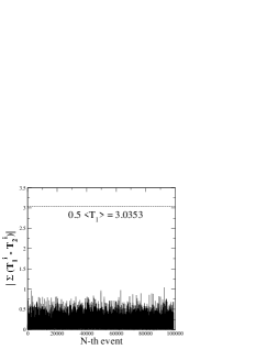
Figure 1: The fluctuation $|\sum_{i=0}^{N}(T^{i}_{1}-T^{i}_{2})|$, in Eq. (9). Note that $|\sum_{i=0}^{N}(T^{i}_{1}-T^{i}_{2})|$ $\leq 0.5\langle T_{1}\rangle$. $\delta\alpha=0.001$ and $\epsilon$=0.01. The phase is calculated from Eq. (3).

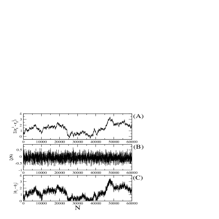
Figure 2: In (A), we show the phase difference at the time the $N$-th event happens in both subsystems. In (B) we show $\xi(N)$, and in (C), we show the phase difference, at the time that the $N$-th event happens in $\mathcal{X}_{1}$. So, the number of events in $\mathcal{X}_{2}$, $N_{2}$, can assume either one of the following values $(N-1,N,N+1)$. $\delta\alpha=0.001$ and $\epsilon$=0.01. The phase is calculated from Eq. (3)

In Fig. 2(A), we show the phase difference at the time the $N$-th event happens in both systems, i.e. the term $\sum_{i=0}^{N}(r^{i}_{1}-r^{i}_{2})$ in Eq. (11). Note that the time that the $N$-th event happens in $\mathcal{X}_{1}$ is different that the time the $N$-th event happens in $\mathcal{X}_{2}$. In (B), we show $\xi(N)$ in Eq. (12), and in (C), we show the phase difference, at the time that the $N$-th event happens in $\mathcal{X}_{1}$. Note that the phase difference in (C) is just the phase difference for the same number of events [in (A)] plus the term $\xi(N)$ [in (B)].

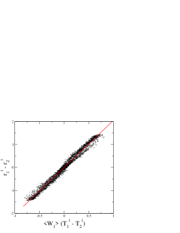
Figure 3: The variable $r_{1}^{i}-r_{2}^{i}$ versus $\langle W_{1}\rangle(T_{1}^{i}-T_{2}^{i})$. We find that $r_{1}^{i}-r_{2}^{i}\simeq\beta\langle W_{1}\rangle(T_{1}^{i}-T_{2}^{i})$, with $\beta$ = 2.0512(3).

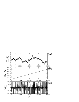
Figure 4: In (A), we show the quantity $\sigma$ in Eq. (17) for a situation when PS exists. As we decrease the coupling, Eq. (20) is not anymore satisfied as shown in (B), as well as Eq. (17), as shown in (C). In (C) we have made a zoom in of the vertical axis. In (A), $\delta\alpha=0.001$ and $\epsilon$=0.01 and in (B-C), $\delta\alpha=0.001$ and $\epsilon$=0.000001.

Then, we show in Fig. 3 that the linear hypothesis between $r_{1}^{i}-r_{2}^{i}$ and $\langle W_{1}\rangle(T_{1}^{i}-T_{2}^{i})$ done in Eq. (13) stands and $\beta$=2.0512$\pm$0.0003. If PS is not present, such linear scale is not anymore found for the system considered.

In Fig. (4)(A), we show the quantity $\sigma$ in Eq. (17) for a situation that PS exists. As we decrease the coupling, Eq. (20) is not anymore satisfied as shown in (B), as well as, Eq. (17). In (C) we make a zoom in of the vertical axis. Note the different nature of the fluctuations of the phase difference in (B) and the term $\sigma$ in Eq. (17). That is because the term $\sigma$ represents the phase difference without the linear growing trend, responsible to make the phase difference in (B) to present a positive slope.

In order to compare the phase as defined in Eq. (3) (for $\delta\alpha$=0.001 and $\epsilon$=0.01), and the phase as defined in park , e.g. $\theta=tg(y/x)$, we compare the function $\langle r_{j}\rangle$, as calculated for both definitions. For the phase, as defined in Eq. (3), we arrive at $\langle r_{j}\rangle$=6.2984 and so, $\langle r_{j}\rangle>2\pi$. Other quantities are $\langle W_{j}\rangle$=0.1651, and $\langle T_{j}\rangle$ = 6.07097. On the other hand, the phase as defined in park is a function that grows in average 2$\pi$ each time the trajectory crosses some Poincaré section, which gives $\langle r_{j}\rangle=2\pi$. So, the phase definitions arrive at two different quantities, but Eq. (20) is valid in order to detect PS and Eq. (6) is valid to measure the average angular frequency of the attractor, using both phase definitions.

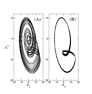
Figure 5: Chaotic attractors projected on the variables $x_{1}$ and $y_{1}$. (A) The coupling is null and therefore, there is no PS. Here one sees the non-coherent Fannel attractor. (B) The coupling induces PS, creating a coherent dynamics.

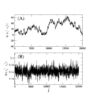
Figure 6: Discrete phase difference $|\sum_{i=0}^{N-1}(r^{i}_{1}-r^{i}_{2})|$ for no coupling (A) where there is not PS and for a coupling $\epsilon$ = 0.00535 (B) responsible to induce PS.

To illustrate the generality of the phase definition in Eq. (3) in order to detect the phenomena of PS in non-coherent attractors, we consider Eqs. (21) with the following set of parameters, $a$=0.3, $b$=0.4, $d$=7.5, such that we have the fannel attractor shown in Fig. 5(A). This attractor has a non-coherent phase character osipov ; kreso . For a parameter mismatch of $\delta\alpha=0.0002$, and for a null coupling, $\epsilon$=0, both Rössler oscillators (presenting the fannel attractor) are not phase synchronized as one can check in Fig. 6(A), which shows the absolute discrete phase difference in Eq. (19). As we introduce the coupling $\epsilon$ = 0.00535, the oscillators presents weak coherent motion.

IV Phase synchronization in two coupled neurons

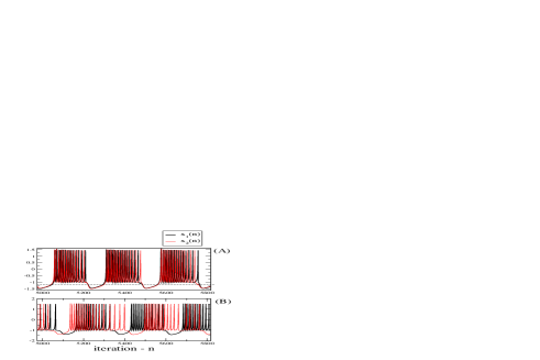
Figure 7: A sample of the variables $x_{1}(n)$ and $x_{2}(n)$, from the subspaces that correspond to both neurons, for a situation where there is PS, for $\epsilon$=0.03 (A), and for a situation where there is not PS, for $\epsilon$=0.001 (B). In (A), Eq. (9) is satisfied, and in (B) is not. In (A), we show three bursts, which are basically a sequence of spiking.

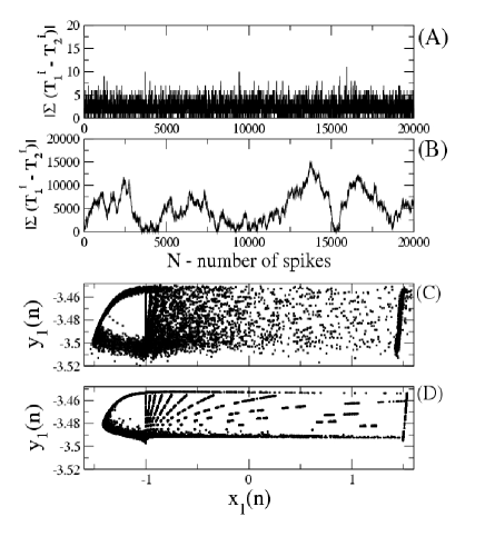
Figure 8: In (A-B), we show the absolute difference between the time of the $N$-th burst, in both subspaces (that represent the two neurons). In (A), Eq. (9) is satisfied with $\langle T_{1}\rangle$=259.028 and, in (B), Eq. (9) is not satisfied (there is not PS). For (A) and (C), $\alpha_{1}$=4.99 and $\epsilon$=0.03. For (B) and (D), $\alpha_{1}$=4.99 and $\epsilon$=0.001.

Now, we give an example for the detection of PS without the knowledge of the state equations, but either only using a time series of bursting events. We consider two non-identical coupled neurons described by

$$x_{j}({n+1}) = f[x_{j}(n),y_{j}(n)+\beta_{j}(n)]$$ (22)

$$y_{j}({n+1}) = y_{j}(n)-\theta(x_{j}({n})+1)+\theta\sigma_{j}+\theta\beta_{j}(n),$$ (23)

which produces a chaotic attractor, for $\theta$ = $0.001$, $\alpha_{2}$=5, $\sigma_{1}=0.240$, and $\sigma_{2}$=0.241. The subspaces are defined as $\mathcal{X}_{j}$=$({x_{j},y_{j}})$. $\beta_{1,2}(n)$ = $g[x_{2,1}(n)-x_{1,2}(n)]$. The function $f$ is given by

$$f=\alpha_{j}/[1-x_{j}(n)]+y_{j}(n),\mbox{\ \ \ }x\leq 0$$

$$f=\alpha_{j}+y_{j}(n),\mbox{\ \ \ }0<x<\alpha_{j}(n)+y$$ (24)

$$f=-1,\mbox{\ \ \ }x\geq\alpha+y_{j}(n)$$

The control parameters are $\alpha_{1}$ and $g$, with $|\alpha_{1}-\alpha_{2}|$ being the parameter mismatch and $g$ the coupling amplitude (cf. rulkov ). The time at which events occur is defined by measuring the time instants in which the variable $x_{j}$, of subsystem $\mathcal{X}_{j}$, is equal to $x_{j}=-1.2$ (the event is the occurrence of a burst) explica_threshold , and $N_{j}$ is the number of bursts of the subsystem $\mathcal{X}_{j}$. In this example, PS exists if Eq. (9) is satisfied, which also means that Eq. (7) is satisfied.

In Fig. 7, we show the variables $x_{1}(n)$ and $x_{2}(n)$ for a situation where there is PS (A), and for a situation where there is not PS (B). Note that in (A), although the neurons are phase synchronized, the difference between the number of bursts in the variable $x_{1}(n)$ minus the number of bursts in the variable $x_{2}(n)$ might be different than zero (for a short moment), as the hypothesis done in Eq. (7). In (A), we also represent by the dashed line the threshold, $x_{j}=-1.2$, from which the events are specified.

In Fig. 8(A-B), we show the absolute difference between the time of the $N$-th burst, in both neurons. In (A), Eq. (9) is satisfied (there is PS) with $\langle T_{1}\rangle$=259.028, and therefore 0.5$\langle T_{1}\rangle$=124.5014, much bigger than the maximum fluctuation in (A). In (B), there is no PS. In (C) and (D), we show a projection of the attractor on the variables $(x_{1},y_{1})$. In (B) and (D), $\langle T_{1}\rangle$ = 396.964, and $\langle T_{2}\rangle$ = 398.407.

Note that although the attractor of these neurons have not the dynamics of a limit cycle, presenting a very complicated geometry in the phase space (as one can see in Fig. 8), it is still possible to well define events as well as the average period of the spiking times by the use of the threshold shown in Fig. 7, a characteristic that defines this attractor to be of the weak coherent type.

V Conclusions

We estimate the inferior bound value of the absolute phase difference between two coupled chaotic systems, in order to verify the existence of phase synchronization between them. Our approach shows that this bound value $\langle r\rangle$ is given by the average evolution of the phase, calculated in a subspace of the attractor, for a series of pairs of events in this same subspace. These events can be the number of local maxima or minima in the trajectory, the crossing of the trajectory to some Poincaré section, or the occurrence of a burst/spike.

This result was achieve because we can inspect for phase synchronization looking for the phase difference at the times for which the same number of events happens in both subsystems. The advantage of looking at the phase difference at these times, instead of looking at the continuous phase difference, is that this approach allows us to detect phase synchronization by looking for a bounded time difference between events. This is helpful for chaotic systems from which there is no available information about the state equations.

If only the number of events is available, one can also find evidences of PS by checking that the absolute difference between the number of events has to be smaller or equal than 1. This allows to infer the existence of PS in maps. These maps can be derived either from a flow (by measuring events as the trajectory crosses a Poincaré section, or by detecting local maxima of the trajectory) or they can be dynamical systems with a discrete formulation.

In this work, the phase is introduced to be a quantity that measures the amount of rotation of the tangent vector of the flow.

All our results are extended to coupled chaotic systems that present coherent properties as defined in kreso , i.e., it is possible to define an average time between two events $\langle T\rangle$, such that for each returning time $\tau$, it is true that $|\tau-\langle T\rangle|<\kappa$, with $\kappa\ll\langle T\rangle$.

VI Acknowledgment

MSB would like to thank Alexander von Humboldt Foundation. TP and JK would like to thank the Helmholz Center for Mind and Brain Dynamics and SFB 555.

Appendix A Contructing PS-sets from the event time series

The event time series $\tau_{j}^{i}$ can be used to construct maps of the attractor, whose geometrical properties states whether there is PS. These maps are constructed following simple rules:

• At the time $\tau_{2}^{i}$, a point of the trajectory in $\mathcal{X}_{1}$ is collected.

• At the time $\tau_{1}^{i}$, a point of the trajectory in $\mathcal{X}_{2}$ is collected.

So, as a result of measuring the trajectories in $\mathcal{X}_{1}$ (resp.$\mathcal{X}_{2}$) at the times $\tau_{2}^{i}$ (resp $\tau_{1}^{i}$) we have a discret set of points $\mathcal{D}_{1}$ ( resp. $\mathcal{D}_{2}$).

In PS, these sets $\mathcal{D}_{j}$ will be localized, not spreading out to the whole attractor. In this case $\mathcal{D}_{j}$ is called PS-set. The theory for characthering and constructing these sets is presented in baptista:2004 . In a short, what happens is the following: when phase synchronization occurs, the times for a trajectory to pass through a Poincare section (or reach some defined event) becomes relatively more regular. Since we measure the trajectory on $\mathcal{X}_{1}$ by the timing of events in $\mathcal{X}_{2}$, these maps are localized around the Poincaré section. For a non synchronous phase dynamics, the sets $\mathcal{D}_{j}$ spreads over $\mathcal{X}_{j}$. Thus, by detecting a PS-set, one does not have to check if the inequality for the time event difference holds.

In the following, we give examples of the PS-sets in the coupled Rössler oscillators and in the Rulkov map, that mimics the neuronal dynamics presenting spiking/burting behavior.

A.1 PS-sets for the coupled Rössler oscillators

The time series, $\mathcal{M}^{\tau}_{j}$, that define the events in $\mathcal{X}_{j}$, are defined as follows. $\mathcal{M}^{\tau}_{1}$: $\tau^{i}_{1}$ is constructed measuring the time the trajectory crosses the plane $y_{2}$=0 in $\mathcal{X}_{2}$; $\mathcal{M}^{\tau}_{2}$: $\tau^{i}_{2}$ is constructed measuring the time the trajectory crosses the plane $y_{1}$=0 in $\mathcal{X}_{1}$.

In Fig. 9, we show the coupled Rössler oscillators for a situation where PS exists. In this figure, we show bidimensional projections on the variables of subsystem $\mathcal{X}_{2}$ (A) and $\mathcal{X}_{1}$ (B). In gray, we show the attractor projection, and in black, projections of the PS-set $\mathcal{D}_{1}$ (A) and $\mathcal{D}_{2}$ (B). Note that the PS-sets, do not visit everywhere $\mathcal{X}_{j}$, rather are localized structures.

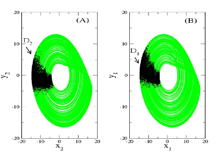
Figure 9: Bidimensional projection of the attractor (gray) and of the projections $\mathcal{D}_{j}$ of the PS-set (black) on the subspaces $\mathcal{X}_{j}$. The PS-set projection $\mathcal{D}_{2}$, in (A), is constructed using time series $\mathcal{M}^{\tau}_{2}$, and $\mathcal{D}_{1}$, in (B), is constructed using time series $\mathcal{M}^{\tau}_{1}$. $\delta\alpha=0.001$ and $\epsilon$=0.01.

A.2 PS-sets for the coupled Rulkov Map

In the neuronal dynamics is not possible to define a Poincaré section, due to the non-coherence of the attractor. However, it is possible to define an event where the dynamics is weak coherent. This event is the ending or the beggining of the bursts, and in here we choose the beggining of the burst. Hence, we construct our time series by measuring the crossing of the trajectory with the threshold, $x_{j}=-1.2$.

In Fig. 10 we show a projection of the attractor on the variables $(x_{1},y_{1})$, in black points, and the subsets $\mathcal{D}_{j}$, in gray points. In (A), where we have phase synchronization the set $\mathcal{D}_{1}$ does not fullfil the whole attractor, but is rather localized, whereas in (B), where PS is not present the set $\mathcal{D}_{2}$ spreads over the attractor $\mathcal{X}_{2}$.

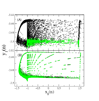
Figure 10: In (A-B), we show the absolute difference between the time of the $N$-th burst, in both subspaces (that represent the two neurons). In (A), Eq. (9) is satisfied (there is PS), with $\langle T_{1}\rangle$=259.028 and, in (B), Eq. (9) is not satisfied (there is not PS). For the same parameters as in (A), in (C) we show the PS-set projection $\mathcal{D}_{1}$ (gray), while for the same parameters as in (B), in (D) there is not a PS-set. For (A) and (C), $\alpha_{1}$=4.99 and $\epsilon$=0.03. For (B) and (D), $\alpha_{1}$=4.99 and $\epsilon$=0.001.

Appendix B $\beta$ digression

In this section we explain why in coherent attractors, e.g. Rössler-type, the constant $\beta$ is approximately 2.

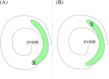
Figure 11: Pictorial visualization of a situation where PS exists. We represent in (A) the trajectory in the subspace $\mathcal{X}_{1}$, and (B) the trajectory in the subspace $\mathcal{X}_{2}$. The filled regions in (A) [(B)] represent trajectory positions at the time the $N$-th event happens in $\mathcal{X}_{2}$ [$\mathcal{X}_{1}$] for a situation when PS exists. An event is considered to happen when the trajectory crosses the dotted line.

That is so, because we compare the phase difference at the time events occurrence. Let us just remember that we are measuring the phase in one subsystem at the times that events in the other subsystem happen. Hence, at the time events happens in $\mathcal{X}_{1}$ [resp. $\mathcal{X}_{2}$], we collect points in $\mathcal{X}_{2}$ [resp. $\mathcal{X}_{1}$], obtaining the gray filled region in Fig. 11(B) [resp. (A)], which is a PS-set.

In particular, when the $N$-th event happens in $\mathcal{X}_{2}$, the trajectory on $\mathcal{X}_{1}$ is indicated by the cross in (A). At this time, $\tau_{2}^{N}$, we record the phase in $\mathcal{X}_{1}$, namely $\phi_{1}(\tau_{2}^{N})$. As the time goes on, the trajectory (in a unclockwise direction of rotation) on $\mathcal{X}_{1}$ reaches the event line in $\mathcal{X}_{2}$ at the time $\tau_{1}^{N}$. At this time, the trajectory in $\mathcal{X}_{2}$ is at the cross in (B), and the phase is $\phi_{2}(\tau_{1}^{N})$. Since these are typical events, we can say that $|\tau_{2}^{N}-\tau_{1}^{N}|\approx\langle T\rangle/4$, for the particular case represented in this figure. That is so because the time difference is approaximately given by the time that the trajectory in $\mathcal{X}_{1}$ spends from the cross in (A) till the event line, which is approximately 1/4 of the average period $\langle T\rangle$.

The phase difference, at which the same number $N$ of events happen, is $|\phi_{1}(\tau_{1}^{N})-\phi_{1}(\tau_{2}^{N})|\approx\langle r\rangle/2$, since this phase difference is basically given by the displacement of the phase in $\mathcal{X}_{1}$ from the cross in (A) till the event line, plus, the displacement of the phase in $\mathcal{X}_{2}$ from the event line till the cross in (B). But that is approximately given by 1/2 of the average increasing of the phase $\langle r\rangle$, which was shown to be equal to $\langle W\rangle\times\langle T\rangle$. Therefore, $|\phi_{1}(\tau_{1}^{N})-\phi_{1}(\tau_{2}^{N})|\approx 2\times|tau_{2}^{N}-\tau_{1}^{N}|$, which consequently give us that $\beta\approx 2$.

References

- (1) A. Pikovsky, M. Rosenblum, and J. Kurths, Synchronization: A Universal Concept in Nonlinear Sciences, (Cambridge University Press, 2001); S. Boccaletti, J. Kurths, G. Osipov, D. Valladares, and C. Zhou, Phys. Rep. 366 (2002) 1; J. Kurths, S. Boccaletti, C. Grebogi, et al. Chaos 13 (2003) 126.
- (2) M.G. Rosenblum, A.S. Pikovsky, and J. Kurths, Phys. Rev. Lett. 76 (1996) 1804; E. Rosa, Jr., E. Ott, and M. H. Hess Phys. Rev. Lett. 80 (1998) 1642; E.-H. Park, M. A. Zaks, and J. Kurths, Phys. Rev. E 60 (1999) 6627.
- (3) U. Parlitz, L. Junge, W. Lauterborn, and L. Kocarev, Phys. Rev. E 54 (1996) 2115.
- (4) I. Z. Kiss and J. L. Hudson, Phys. Rev. E, 64 (2001) 046215.
- (5) C. M. Ticos, E. Rosa, Jr., and W. B. Pardo, et al., Phys. Rev. Lett. 85 (2000) 2929.
- (6) M. S. Baptista, T. Pereira, J. C. Sartorelli, I. L. Caldas, and E. Rosa, Jr. Phys. Rev. E 67 (2003) 056212.
- (7) J. Fell, P. Klaver. C. E. Elger, and G. Fernandez, Rev. Neurosc. (2002) 13 299.
- (8) F. Mormann, T. Kreuz, R. G. Andrzejak, P. David, K. Lehnertz, and C. E. Elger, Epilepsy Research 53 (2003) 173.
- (9) is considered to be a rational. However, as shown in Ref. murilo , PS, as defined by the boundness of the phase difference was found in two chaotic systems for a finite but very large time interval, as approaches an irrational. Therefore, although in this work we consider to be rational, we should make the remark that for the especial situation as the one presented in Ref. murilo , Eq. (20) can only be satisfied for a finite but large time if is considered to be irrational.
- (10) M. S. Baptista, S. Boccaletti, K. Josić, and I. Leyva, Phys. Rev. E 69 (2004) 056228.
- (11) In Eq. (1), we assume that the coupled system reached equilibrium, i.e., the asymptotic dynamics. Otherwise, one could introduce another finite constant inside the left side of this equation.
- (12) Phase can be defined as a Hilbert transformation of a trajectory component, as the angle of a trajectory point into a special projection of the attractor, or as a function that grows , every time the chaotic trajectory crosses some specific surface. In this work, we define phase to be a measure of the absolute rotation of the tangent vector in the subspaces .
- (13) M. S. Baptista, T. Pereira, J. C. Sartorelli, and I. L. Caldas, “Non-transitive transformations in phase synchronization”, to be published in Physica D.
- (14) N. F. Rulkov, Phys. Rev E 65 (2002) 041922.
- (15) A trivial case, where can be analytically computed is in a planar circular motion. The position vector is , and the unitary tangent vector has the coordinates . The derivative of the tangent vector has the coordinates , and therefore, =, and = .
- (16) In Ref. jalan:2003 , PS is defined by the difference between the number of events being equal to zero. More precisely, . But, this assumption is too strong to detect PS, once that the trajectories of phase synchronous systems may be uncorrelated. So, the difference between events might differ by an unit, in a generical case.
- (17) R. D. Pinto, W. M. Gonçalves, J. C. Sartorelli, I. L. Caldas, M. S. Baptista, Phys. Rev. E, 58 4009 (1998).
- (18) S. P. Strong, R. Koberle, R. R. D. van Steveninck, et al. Phys. Rev. Lett. 80, 197 (1998).
- (19) S. Jalan and R. E. Amritkar, Phys. Rev. Lett. 90 (2003) 014101.
- (20) K. Josić and M. Beck, Chaos 13 (2003) 247; K. Josić and D. J. Mar, Phys. Rev. E 64 (2001) 056234.
- (21) V. G. Osipov, H. Bambi, C. Zhou, V. M. Ivanchenko, and J. Kurths. Phys. Rev. Lett. 91 (2003) 024101.
- (22) This threshold enables to detect the time at which a burst starts. In fact, due to small fluctuations of the trajectory close to the used threshold, =-1.2, we only consider that a burst starts (the event happened), if after the trajectory having crossed the threshold at =-1.2, it crosses eventually another threshold, positioned in =0, before it crosses again the threshold =-1.2, in the next event.