Hydrodynamic Model for the System of Self Propelling Particles with Conservative Kinematic Constraints; Two dimensional stationary solutions

Abstract

In a first paper we proposed a continuum model for the dynamics of systems of self propelling particles with kinematic constraints on the velocities. The model aims to be analogous to a discrete algorithm used in works by T. Vicsek et al. In this paper we prove that the only types of the stationary planar solutions in the model are either of translational or axial symmetry of the flow. Within the proposed model we differentiate between finite and infinite flocking behavior by the finiteness of the kinetic energy functional.

1 Introduction

The dynamics of systems of particles subjected to nonpotential interactions remains poorly understood. The absence of a Hamiltonian for such systems, which generally are far from equilibrium, hampers applying the machinery of statistical mechanics based on the Liouville equation. Many attempts have been made to investigate these systems using discrete algorithms to model this behavior. In nature there are many examples of such systems [1]. Since the discrete algorithms are hard to describe analytically it is natural also to consider continuum models of a hydrodynamic type. In standard hydrodynamics the relation between microscopic kinetics (Boltzmann-type equations) and Navier-Stokes equations is a standard topic of research [2]. For the systems of interest the construction of corresponding kinetic equations based on the specific dynamic rules and their connection with the hydrodynamics equations seems to be unknown so far and is worth studying. One can expect that the continuous description of the collective behavior like swarming and flocking leads to quite unusual hydrodynamics.

In our first paper [3] we proposed a hydrodynamic model which can be considered to be the continuum analogue of the discrete dynamic automaton proposed by Vicsek et al. [4] for a system of self propelling particles. It uses the continuity equation

$$\frac{\partial n(\mathbf{r},t)}{\partial t}+\mathop{\rm div}\nolimits\left(n(\mathbf{r},t)\,\mathbf{v}(\mathbf{r},t)\right)=0\,,$$ (1)

which implies that the total number of particles

$$N=\int n(\mathbf{r},t)\,d\mathbf{r}$$ (2)

is constant. The kinetic energy of a co-moving volume

$$T=\frac{1}{2}\int n(\mathbf{r},t)\mathbf{v}^{2}(\mathbf{r},t)d\mathbf{r}$$ (3)

is also conserved

$$\frac{d}{dt}T=0\,.$$ (4)

Using Eq. (1) and Eq. (4) it can be shown that a field $\boldsymbol{\omega}$ exists such that the Eulerian velocity, $\mathbf{v}(\mathbf{r},t),$ satisfies:

$$\frac{d}{dt}\mathbf{v}\left(\mathbf{r},t\right)=\boldsymbol{\omega}\left(\mathbf{r},t\right)\times\mathbf{v}\left(\mathbf{r},t\right).$$ (5)

This equation can be considered as the continuous analogue of the conservative dynamic rule used by Vicsek et al. [4].

We proposed the following “minimal“ model for the field of the angular velocity $\boldsymbol{\omega}\left(\mathbf{r},t\right)$ which is linear in spatial gradients of the fields $n(\mathbf{r},t)$ or $\mathbf{v}(\mathbf{r},t)$:

$$\mathbf{\omega}\left(\mathbf{r},t\right)=\int K_{1}\left(\mathbf{r}-\mathbf{r^{\prime}}\right)\,n(\mathbf{r^{\prime}},t)\mathop{\rm rot}\nolimits\mathbf{v}(\mathbf{r^{\prime}},t)\,d\mathbf{r^{\prime}+}\int K_{2}\left(\mathbf{r}-\mathbf{r^{\prime}}\right)\nabla n\left(\mathbf{r^{\prime}},t\right)\times\mathbf{v}(\mathbf{r^{\prime}},t)d\mathbf{r^{\prime}}\,.$$ (6)

$\boldsymbol{\omega}$ has the proper pseudovector character. The averaging kernels $K_{1}\left(\mathbf{r}-\mathbf{r^{\prime}}\right)$ and $K_{2}\left(\mathbf{r}-\mathbf{r^{\prime}}\right)$ should naturally decrease with the distance in realistic models. They sample the density and the velocity around $\mathbf{r}$ in order to determine $\boldsymbol{\omega}\left(\mathbf{r},t\right)$. In the first paper we concentrated on $K_{1}$. The detailed derivation of the above equations from the discrete models based on the automaton proposed by Vicsek et al. [4, 5] will be the subject of a future paper.

Note that the models based on Eqs. (1)-(6) allow solutions of uniform motion in the form of a solitary packet:

$$n(\mathbf{r},t)=n_{0}(\mathbf{r}-\mathbf{v}_{0}\,t)$$ (7)

with $\mathbf{v}_{0}$ independent of position and time. The contribution to $\boldsymbol{\omega}$ due to $K_{1}$ is zero for an arbitrary density distribution $n_{0}$. The contribution due to $K_{2}$ is zero for density distributions $n_{0}$ which only depend on the position in the $\mathbf{v}_{0}$ direction. In this second case it follows from the continuity equation that $n_{0}$ should be everywhere constant. The density distribution $n_{0}$ should be chosen such that the number of particles, and, correspondingly, the total kinetic energy are finite. The solutions of such type also were found analytically in [6] and observed in simulations [7]. Note that such solutions exist not only in nonlocal case like in [6] but also for the local model which we consider below.

Within the first order of perturbation theory on small deviation of density and velocity fields the solitary solution given by Eq. (7) shows neutral stability; i.e. the perturbations grows linearly for small $t$.

We restrict our discussion to the simple case of averaging kernels, which are $\delta$-functions:

$$K_{j}\,(\mathbf{r}-\mathbf{r}^{\prime})=s_{j}\,\delta(\mathbf{r}-\mathbf{r}^{\prime})\,,\quad\text{\ where \ \ }j=1\text{ or 2}.$$ (8)

We will call this the local hydrodynamic model (LHM). In the first paper, where we only considered $K_{1}$, we scaled $K_{1}$ by dividing by $\left|s_{1}\right|$ and the density $n$ by multiplying with $\left|s_{1}\right|$. This made it then possible to restrict the discussion to $s_{1}$ is plus or minus one. The disadvantage of this scaling procedure is that it changes the dimensionality of $K_{j}$ and $n$. For two kernels it becomes impractical. We note that $s_{j}$ is given by:

$$s_{j}=\int\ K_{j}\left(\mathbf{r}\right)d\mathbf{r}.$$ (9)

For the local model Eq.(6) reduces to:

$$\boldsymbol{\omega}\left(\mathbf{r},t\right)=s_{1}\,n(\mathbf{r},t)\mathop{\rm rot}\nolimits\mathbf{v}(\mathbf{r},t)\text{ }\mathbf{+}\text{ }s_{2}\mathbf{\nabla}n\left(\mathbf{r},t\right)\times\mathbf{v}(\mathbf{r},t).$$ (10)

and Eq. (5) for the velocity becomes

$$\frac{d}{dt}\mathbf{v}\left(\mathbf{r},t\right)=s_{1}\,n(\mathbf{r},t)\mathop{\rm rot}\nolimits\mathbf{v}(\mathbf{r},t)\times\mathbf{v}\left(\mathbf{r},t\right)+s_{2}\left(\mathbf{\nabla}n\left(\mathbf{r},t\right)\times\mathbf{v}(\mathbf{r},t)\right)\times\mathbf{v}\left(\mathbf{r},t\right)\,.$$ (11)

Note that the second term on the right-hand-side of Eq. (11) corresponds to the rotor chemotaxis force when the number density is proportional to the attractant density introduced in [5].

In the following section we will show that the only stationary solutions for LHM with $\boldsymbol{\omega}$ field given by Eq. (10) are either the solutions of uniform motion (see Eq. (7)) or the radially symmetric planar solution which will be considered in detail in the following section.

In the second section we investigate the properties of the stationary radially symmetric solutions of the local hydrodynamic model for some special cases. Conclusions are given in the last section.

2 Possible types of stationary states for the local hydrodynamical model

The equations of motion to be solved are Eqs. (1) and  (11). In order to find a class of 2D stationary solutions we consider this problem in a generalized curvilinear orthogonal coordinate system $(u,v)$, which can be obtained from the Cartesian one $(x,y)$ by some conformal transformation of the following form:

$$u+iv=F\left(z\right),$$ (12)

where $F(z)$ is an arbitrary analytical function of $z=x+iy$. In a curvilinear orthogonal coordinate system the fundamental tensor has a diagonal form, $g_{ik}=g_{ii}\delta_{ik}$, where the indices $i,j$ are either $u$ or $v$. The square of linear element in conformal coordinates is

$$d\mathbf{s}^{2}=\frac{1}{D(u,v)}\left(du^{2}+dv^{2}\right),$$ (13)

where

$$D(u,v)=\frac{\partial\left(u,v\right)}{\partial\left(x,y\right)}=\left(\frac{\partial u}{\partial x}\right)^{2}+\left(\frac{\partial u}{\partial y}\right)^{2}=\left(\frac{\partial v}{\partial x}\right)^{2}+\left(\frac{\partial v}{\partial y}\right)^{2}=\frac{1}{\sqrt{g}}$$ (14)

is the Jacobian of the inverse conformal transformation from the arbitrary curvilinear orthogonal to Cartesian coordinates, $(u,v)\rightarrow(x,y)$. Furthermore $g=g_{uu}g_{vv}$ is the determinant of the metric tensor. For a conformal transformation $g_{vv}=g_{uu}=1/D$.

The differential operations are given by the following expressions [8]:

$$\nabla\phi = \sqrt{D}\left(\mathbf{e}_{u}\frac{\partial\phi}{\partial u}+\mathbf{e}_{v}\frac{\partial\phi}{\partial v}\right),$$ (15)

$$\mathop{\rm div}\nolimits\mathbf{a} = D\left[\frac{\partial}{\partial u}\left(\frac{a_{u}}{\sqrt{D}}\right)+\frac{\partial}{\partial v}\left(\frac{a_{v}}{\sqrt{D}}\right)\right],$$ (16)

$$\mathop{\rm rot}\nolimits\mathbf{a} = D\left[\frac{\partial}{\partial u}\left(\frac{a_{v}}{\sqrt{D}}\right)-\frac{\partial}{\partial v}\left(\frac{a_{u}}{\sqrt{D}}\right)\right],$$ (17)

$$\Delta\phi = D\left[\frac{\partial^{2}\phi}{\partial u^{2}}+\frac{\partial^{2}\phi}{\partial v^{2}}\right]\,.$$ (18)

Here $\mathbf{e}_{u}$ and $\mathbf{e}_{v}$ are orthonormal base vectors in the directions of increasing $u$ and $v$ respectively. These base vectors are functions of the coordinates $u$ and $v$. The projections of the vectorfield $\mathbf{a}$ on these directions are $a_{u}=\mathbf{a\cdot e}_{u}$ and $a_{v}=\mathbf{a\cdot e}_{v}$. Using Eqs. (15)-(18) for the velocity field given by $\mathbf{v}=\mathrm{v}_{u}\,\mathbf{e}_{u}+\mathrm{v}_{v}\,\mathbf{e}_{v}$, one obtains:

$$\left(\mathbf{v}\cdot\nabla\right)\,\mathbf{v}=\sqrt{D}\left[\mathrm{v}_{u}\frac{\partial(\mathrm{v}_{u}\mathbf{e}_{u})}{\partial u}+\mathrm{v}_{v}\frac{\partial(\mathrm{v}_{u}\mathbf{e}_{u})}{\partial v}+\mathrm{v}_{u}\frac{\partial(\mathrm{v}_{v}\mathbf{e}_{v})}{\partial u}+\mathrm{v}_{v}\frac{\partial(\mathrm{v}_{v}\mathbf{e}_{v})}{\partial v}\right],$$ (19)

$$\mathop{\rm rot}\nolimits\mathbf{v}\times\mathbf{v}=D\left[\frac{\partial}{\partial u}\left(\frac{\mathrm{v}_{v}}{\sqrt{D}}\right)-\frac{\partial}{\partial v}\left(\frac{\mathrm{v}_{u}}{\sqrt{D}}\right)\right](-\mathrm{v}_{v}\mathbf{e}_{u}+\mathrm{v}_{u}\mathbf{e}_{v}),$$ (20)

$$\left(\mathbf{\nabla}n\times\mathbf{v}\right)\times\mathbf{v=}\sqrt{D}\left[\frac{\partial n}{\partial u}\mathrm{v}_{v}-\frac{\partial n}{\partial v}\mathrm{v}_{u}\right]\left(-\mathrm{v}_{v}\mathbf{e}_{u}+\mathrm{v}_{u}\mathbf{e}_{v}\right),$$ (21)

$$\mathop{\rm div}\nolimits(n\mathbf{v})=D\left[\frac{\partial}{\partial u}\left(\frac{n\mathrm{v}_{u}}{\sqrt{D}}\right)+\frac{\partial}{\partial v}\left(\frac{n\mathrm{v}_{v}}{\sqrt{D}}\right)\right]=0.$$ (22)

Substituting Eqs. (19)-(22) into Eqs. (1) and (11) we obtain the following system of equations, which determines all possible stationary flows for the LHM:

$$\mathrm{v}_{u}\frac{\partial\mathrm{v}_{u}}{\partial u}+(1-s_{1}n)\mathrm{v}_{v}\frac{\partial\mathrm{v}_{u}}{\partial v}+\mathrm{v}_{u}\mathrm{v}_{v}\left(f_{3}+\frac{s_{1}n}{2}\frac{\partial\ln D}{\partial v}-s_{2}\,\frac{\partial n}{\partial v}\right)+\mathrm{v}_{v}^{2}\left(f_{4}-\frac{s_{1}n}{2}\frac{\partial\ln D}{\partial u}+s_{2}\,\frac{\partial n}{\partial u}\right)+s_{1}n\mathrm{v}_{v}\frac{\partial\mathrm{v}_{v}}{\partial u}=0,$$ (23)

$$\mathrm{v}_{v}\frac{\partial\mathrm{v}_{v}}{\partial v}+(1-s_{1}n)\mathrm{v}_{u}\frac{\partial\mathrm{v}_{v}}{\partial u}+\mathrm{v}_{u}\mathrm{v}_{v}\left(f_{2}+\frac{s_{1}n}{2}\frac{\partial\ln D}{\partial u}-s_{2}\,\frac{\partial n}{\partial u}\right)+\mathrm{v}_{u}^{2}\left(f_{1}-\frac{s_{1}n}{2}\frac{\partial\ln D}{\partial v}+s_{2}\,\frac{\partial n}{\partial v}\right)+s_{1}n\mathrm{v}_{u}\frac{\partial\mathrm{v}_{u}}{\partial v}=0,$$ (24)

$$\frac{\partial}{\partial u}\left(\frac{n\mathrm{v}_{u}}{\sqrt{D}}\right)+\frac{\partial}{\partial v}\left(\frac{n\mathrm{v}_{v}}{\sqrt{D}}\right)=0,$$ (25)

where

$$f_{1}(u,v) = \frac{\partial\mathbf{e}_{u}}{\partial u}\cdot\mathbf{e}_{v}\text{ \ , \ \ }f_{2}(u,v)=\frac{\partial\mathbf{e}_{u}}{\partial v}\cdot\mathbf{e}_{v}$$

$$f_{3}(u,v) = \frac{\partial\mathbf{e}_{v}}{\partial u}\cdot\mathbf{e}_{u}\text{ \ , \ \ }f_{4}(u,v)=\frac{\partial\mathbf{e}_{v}}{\partial v}\cdot\mathbf{e}_{u}$$ (26)

Now let us consider the case of ”coordinate flows”, when the flow is directed along one of the families of coordinate lines $u,v$ for example along $u$-coordinate lines and is given by $\mathbf{v}=(0,\mathrm{v}_{v}(u,v),0)$, the density distribution is $n=n(u,v)$. The case of a velocity field $\mathbf{v}=\mathrm{v}_{u}\mathbf{e}_{u}$ is equivalent (just interchange $u$ and $v$). From Eq. (23) we have:

$$\mathrm{v}_{v}=C\exp\left[\int I(u,v)du\right]\,,$$ (27)

where

$$I(u,v)=\frac{1}{2}\,\frac{\partial\,\ln{D}}{\partial\,u}-\frac{f_{4}}{s_{1}\,n}-\frac{s_{2}}{s_{1}}\frac{\partial\,\ln n}{\partial\,u}\,.$$ (28)

Equations (24) and (25) take the form:

$$\frac{\partial\mathrm{v}_{v}}{\partial v} = 0,$$ (29)

$$\frac{\partial}{\partial v}\left(\frac{n\mathrm{v}_{v}}{\sqrt{D}}\right) = 0$$ (30)

and lead to

$$n(u,v)=h(u)\sqrt{D(u,v)},$$ (31)

where $h(u)$ is an arbitrary function of $u$. Taking into account that:

$$f_{4}(u,v)=\left(\frac{\partial\mathbf{e}_{v}}{\partial v}\cdot\mathbf{e}_{u}\right)=-\frac{D}{2}\frac{\partial\left(1/D\right)}{\partial u}=\frac{1}{2}\frac{\partial\ln D}{\partial u},$$ (32)

and Eq. (31) we obtain:

$$I(u,v)=\frac{1}{2}\,\frac{\partial\,\ln{D}}{\partial\,u}\left[1-\frac{1}{s_{1}\,h(u)\sqrt{D}}-\frac{s_{2}}{s_{1}}\left(2\frac{\partial\,\ln{h(u)}}{\partial\,u}\left(\frac{\partial\,\ln{D}}{\partial\,u}\right)^{-1}+1\right)\right]\,.$$ (33)

Note that as it follows from Eq. (29)

$$\mathrm{v}_{v}(u,v)=\mathrm{v}_{v}(u).$$ (34)

For the integrand in Eq.(27) this implies that

$$I(u,v)=I(u).$$ (35)

Therefore from Eqs. (33) and (35) we can conclude that the function $D(u,v)$, which determines the coordinate system, depends only on one variable, $D=D\,(u)$.

In the case of conformal coordinates, defined by the metrics in Eq. (13), the Gaussian curvature of the surface is given by [9]:

$$K=\frac{1}{2}D\Delta\ln{D}\,.$$ (36)

For a planar flows the condition $K=0$ leads to the following

$$\Delta\ln D=0.$$ (37)

Using the expression for the Laplacian in the conformal representation (see Eqs. (18)) and taking into account a fact that $D=D(u)$ one finds for (37):

$$D=\exp\left[c_{1}u+c_{2}\right],$$ (38)

where $c_{1,2}$ are arbitrary constants. The case $c_{1}=0$ determines a Cartesian coordinate system, which related to a linear class of stationary flow. The case $c_{1}\neq 0$ determines a polar coordinate system [8], which corresponds to an axially symmetric (or vortical) type of flow.

Finally the velocity field for the LHM, with $s_{1}\neq 0$ takes the form:

$$\mathrm{v}_{v}(u)=C\exp\left[\frac{1}{2}\,\int\frac{\partial\,\ln{D}}{\partial\,u}\left[1-\frac{1}{s_{1}\,h(u)\sqrt{D}}-\frac{s_{2}}{s_{1}}\left(2\frac{\partial\,\ln{h(u)}}{\partial\,u}\left(\frac{\partial\,\ln{D}}{\partial\,u}\right)^{-1}+1\right)\right]\,du\right]\,,$$ (39)

Thus it is proved that for the case $s_{1}\neq 0$ the only stationary solutions are those either with planar or axial symmetry of the flow.

The case $s_{1}=0$ (the LM2) is specific because as it follows from Eqs. (23) and (24) the velocity field $v_{v}(u)$ is arbitrary while the density takes the form:

$$n=-\frac{1}{2\,s_{2}}\,\ln{D}+n_{0}\,.$$ (40)

The statement about the symmetry of the stationary solutions for such a model is the same as that proved above for the case $s_{1}\neq 0$. Note that the parameter $\lambda=s_{2}/s_{1}$ can be considered as the weight factor of the rotor chemotaxis contribution.

3 The properties of radially symmetric stationary solutions

In this section we investigate the stationary radially symmetrical solutions for different cases of the local hydrodynamical models. In our first paper we considered the $s_{2}=0$ case, which we called the local model one (LM1). Other models correspond to cases $s_{1}=0$ and $s_{1}=s_{2}=s$ which we will call the LM2 and the LM12 respectively. We consider the finite and infinite flocking stationary states for these models. It is natural to differentiate between these two cases by the finiteness of two integrals of motion - the total number of particles Eq. (2) and the kinetic energy Eq. (4). The infinite flocking is associated with $N$ infinite but finite $T$, while finite flocking naturally corresponds to both $N$ and $T$ finite. Note that in the finite flocking behavior one may consider two cases with respect to the compactness of the $n(r)$. Compactness means that the density has some upper cut-off beyond which it can be put zero.

3.1 The properties of the stationary solutions of LM1

In our previous paper [3] we considered the stationary solutions in LM1 and obtained the for velocity field profile

$$\mathrm{v}_{\varphi}(r)=\frac{C_{1}}{2\pi r}\exp\left(\frac{1}{s_{1}}\int\limits_{r_{0}}^{r}\,\frac{1}{r\,n(r^{\prime})}\,dr^{\prime}\right)\,.$$ (41)

Here $r$ is the radial coordinate and $\varphi$ is the angular one, $r_{0}$ is some radius, which for vortex-like solutions plays the role of lower cut-off radius of the vortex and determines its core.

For vortex-like solutions the constant $C_{1}$ in Eq.(41) is determined by the circulation of the core

$$\oint\limits_{r=r_{0}}\mathbf{v}\cdot d\mathbf{l}=C_{1}.$$ (42)

The spatial character of the solution given in Eq.(41) strongly depends on the sign of the parameter $s_{1}$. The finiteness of integrals of motion Eq. (2) and Eq. (3) is guaranteed by either the fast enough decrease of the density $n(r)$ at $r\to\infty$ or its compactness ($n(r)$ as a function has finite support).

Let us consider the finite flocking behavior (FFB), which is characterized by both $N$ and $T$ finite. If at $r\to\infty$ asymptotically $n(r)\sim r^{-\alpha}$ , where $\alpha>2$ the total number of particles $N$ is finite. Then at such a behavior of $n(r)$ the total kinetic energy is finite only if $s_{1}<0$.

In a case $s_{1}>0$ the condition of finiteness for the kinetic energy and the total number of particles is fulfilled only if $n(r)$ has finite support. As an example we may give:

$$n(r)=n_{1}\theta\left(r-r_{0}\right)\,\theta\left(R-r\right)\sqrt{\frac{r_{0}}{R-r}}\,,\quad n_{1}>0\,,$$ (43)

where $R$ is the upper cut-off radius. Substituting Eq.(43) into Eq.(41) one obtains:

$$\mathrm{v}_{\varphi}(r)=\frac{C_{1}}{2\pi r}\exp\left[\frac{2}{s_{1}n_{1}}\sqrt{\frac{R}{r_{0}}}\left.\left(\sqrt{1-\frac{r}{R}}-\mathop{\rm arctanh}\nolimits\sqrt{1-\frac{r}{R}}\right)\right|_{r_{0}}^{r}\right].$$ (44)

The corresponding profiles for the velocity $\mathbf{v}=\mathrm{v}_{\phi}\,\mathbf{e}_{\phi}$ at different ratio $R/r_{0}$ are shown in Fig. 1. Note that for the case considered at $R/r_{0}\geq 2$ we get the monotonic profiles of the velocity which are similar to those observed in experiments [5].

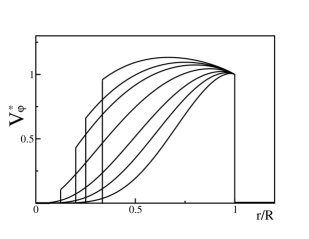
Figure 1: The velocity profiles for ${\rm V}^{*}_{\varphi}=2\pi Rv_{\varphi}(r/R)$ in the LM1 for different ratios $R/r_{0}$ and $s_{1}n_{1}=1$.

The infinite flocking behavior (IFB) is characterized by the $N$ infinite and $T$ finite. For the case $s_{1}>0$ no physical solutions exist with such a behavior. For the case $s_{1}<0$ slowly decaying density distributions $n(r)\propto r^{-\alpha}$ at $r\to\infty$ with $0\leq\alpha\leq 2$ are consistent with the finiteness of $T$. These statements are summed up in Table 1.

LM1	$s_{1}>0$	$s_{1}<0$
FFB $\left(N<\infty,\,T<\infty\right)$	compact support	$\alpha>2$, no compact support
IFB $\left(N=\infty,\,T<\infty\right)$	no physical solutions	$0\leq\alpha\leq 2$

Table 1: Properties of the stationary solutions of the LM1.

3.2 The properties of the stationary solutions of LM2

For the case that $s_{1}=0$ and $s_{2}$ finite one may also construct a radially symmetric stationary planar solution. In polar coordinates from Eq. (40) we get:

$$n(r)=\frac{1}{s_{2}}\ln\frac{r}{r_{0}}\,,$$ (45)

and one can choose the velocity field $\mathrm{v}_{\varphi}(r)$ arbitrarily. For positive values of $s_{2}$ this density is positive for $r>r_{0}$ and for negative values of $s_{2}$ it is positive for $r<r_{0}$. So for positive values of $s_{2}$ the density profile becomes

$$n(r)=\frac{1}{s_{2}}\,\theta\,(R-r)\,\ln\frac{r}{r_{0}}$$ (46)

and for negative values of $s_{2}$ it becomes

$$n(r)=\frac{1}{\left|s_{2}\right|}\,\theta\,(r_{0}-r)\ln\frac{r_{0}}{r}.$$ (47)

The results about finite and infinite flocking behavior are in Table 2.

LM2	$s_{1}>0\,$	$s_{1}<0$
FFB $\left(N<\infty,\,T<\infty\right)$	no physical solution	compact support
IFB $\left(N=\infty,\,T<\infty\right)$	no physical solution	no physical solution

Table 2: Properties of the stationary solutions of the LM2.

3.3 The properties of the stationary solutions of LM12

The third case which is expedient to consider is $s_{1}=s_{2}=s$. In that case, according to Eq. (10), the field $\boldsymbol{\omega}$ is coupled to the number density flux $\mathbf{j}=n\,\mathbf{v}$:

$$\boldsymbol{\omega}\left(\mathbf{r},t\right)=s\,\,\mathop{\rm rot}\mathbf{j}$$ (48)

so that Eq. (11) for the velocity is

$$\frac{d}{dt}\mathbf{v}\left(\mathbf{r},t\right)=s\,\mathop{\rm rot}\mathbf{j}\times\mathbf{v}\left(\mathbf{r},t\right)\,.$$ (49)

For a radially symmetric stationary planar solution this gives

$$\mathrm{v}_{\varphi}(r)=s\frac{d}{dr}\left[rn(r)\mathrm{v}_{\varphi}(r)\right].$$ (50)

with

$$\mathrm{v}_{\varphi}(r)=\frac{C}{2\pi r\,n(r)}\exp\left[\frac{1}{s}\int_{r_{0}}^{r}\frac{1}{r^{\prime}\,n\,(r^{\prime})}\,dr^{\prime}\right]\,.$$ (51)

as a solution. The constant $C$ is determined by the circulation of the core

$$\oint\limits_{r=r_{0}}\mathbf{v}\cdot d\mathbf{l}=\frac{C}{n(r_{0})}\,.$$ (52)

The properties of finite and infinite flocking behavior for this model are the same as those for the LM1 (see Table 1).

4 Conclusions

In this paper we consider the properties of the stationary 2D solutions of the LHM proposed in [3]. We established that the only possible stationary solutions in the model are those with translational or axial symmetry. The cases of finite and infinite flocking behavior are considered for different specific types of the LHM. It is shown that the case $s_{1}=0$ (LM2) is specific in a sense that there is only one density distribution, for which many velocity profiles can be realized. In general case ($s_{1}\neq 0$) one is free to choose axially symmetric density distribution which the velocity profile depends on (Eqs. (31) and (39)). Note that in this respect the general case is similar to the LM1 considered earlier.

References

- [1] J. Parrish, W. Hammer, Animal Groups in Three Dimensions, Cambridge University Press, 1997.
- [2] S. Succi, The Lattice Boltzmann Equation for Fluid Dynamics and Beyond, Clarendon Press, Oxford, 2001.
- [3] V. Kulinskii, V. Ratushnaya, A. Zvelindovsky, D. Bedeaux, Europhys. Lett. 71 (2) (2005) 207.
- [4] T. Vicsek, A. Czirók, E. Ben-Jacob, I. Cohen, O. Shochet, Phys. Rev. Lett. 75 (1995) 1226.
- [5] A. Czirók, E. Ben-Jacob, I. Cohen, T. Vicsek, Phys. Rev. E 54 (1996) 1791.
- [6] C. M. Topaz, A. L. Bertozzi, SIAM J. Appl. Math. 65 (2004) 152.
- [7] G. Grégoire, H. Chaté, Phys. Rev. Lett. 92 (2004) 025702.
- [8] E. Madelung, Die Mathematischen Hilfmittel Des Physikers, Springer Verlag, Berlin, 1964.
- [9] B. Dubrovin, A. Fomenko, S. Novikov, Modern Geometry - Methods and Applications, Springer, 1992.