Earthquake recurrence as a record breaking process

Abstract

Extending the central concept of recurrence times for a point process to recurrent events in space-time allows us to characterize seismicity as a record breaking process using only spatiotemporal relations among events. Linking record breaking events with edges between nodes in a graph generates a complex dynamical network isolated from any length, time or magnitude scales set by the observer. For Southern California, the network of recurrences reveals new statistical features of seismicity with robust scaling laws. The rupture length and its scaling with magnitude emerges as a generic measure for distance between recurrent events. Further, the relative separations for subsequent records in space (or time) form a hierarchy with unexpected scaling properties.

DAVIDSEN, GRASSBERGER AND PACZUSKI Earthquake recurrence J. Davidsen, British Antarctic Survey, High Cross, Madingley Road, Cambridge CB3 0ET, UK. (j.davidsen@bas.ac.uk)

1 Introduction

Fault systems as the San Andreas fault in California or the Sunda megathrust (the great tectonic boundary along which the Australian and Indian plates begin their descent beneath Southeast Asia) are prime examples of self-organizing systems in nature (Rundle et al., 2002). Such systems are characterized by interacting elements, each of which stays quiescent in spite of increasing stress acting on it until the stress reaches a trigger threshold leading to a rapid discharge or ”firing”. Since the internal state variables evolve in time in response to external driving sources and inputs from other elements, the firing of an element may in turn trigger a discharge of other elements. In the context of fault systems, this corresponds to earthquakes, or the deformation and sudden rupture of parts of the earth’s crust driven by convective motion in the mantle.

Fault systems — and driven threshold systems in general — exhibit dynamics that is strongly correlated in space and time over many scales. Their complex spatiotemporal dynamics manifests itself in a number of generic, empirical features of earthquake occurrence including clustering, fault traces and epicenter locations with fractal statistics, as well as scaling laws like the Omori and Gutenberg-Richter (GR) laws (see e.g. Refs. (Turcotte, 1997; Rundle et al., 2003) for a review), giving rise to a worldwide debate about their explanation. Resolving this dispute could conceivably require measuring the internal state variables — the stress and strain everywhere within the earth along active faults — and their exact dynamics. This is (currently) impossible. Yet, the associated earthquake patterns are readily observable making a statistical approach based on the concept of spatiotemporal point processes feasible, where the description of each earthquake is reduced to its size or magnitude, its epicenter and its time of occurrence. Describing the patterns of seismicity may shed light on the fundamental physics since these patterns are emergent processes of the underlying many-body nonlinear system.

Recently, such an approach has brought to light new properties of the clustering of seismicity in space and time (Bak et al., 2002; Corral, 2003, 2004; Davidsen and Goltz, 2004; Davidsen and Paczuski, 2005; Baiesi and Paczuski, 2005), which can potentially be exploited for earthquake prediction (Goltz, 2001; Tiampo et al., 2002; Baiesi, 2006). One aim has been to evaluate distances between subsequent events, including temporal and spatial measures. The observed spatiotemporal clustering of seismicity suggests that subsequent events are to a certain extent causally related. It further suggests that the usual mainshock/aftershock scenario — where each event has at most one correlated predecessor — is too simplistic and that the causal structure of seismicity could extend beyond immediately subsequent events, especially since the determination of the sequence is largely arbitrary depending on the size of the region considered and the completeness of the record of events.

In this work we quantify the spatiotemporal clustering of seismicity in terms of a sparse, directed network, where each earthquake is a node in the graph and links connect events with their recurrences. This general network picture allows us to characterize clustering by using only the spatiotemporal structure of seismicity, without any additional assumptions.

2 Method

The key advance we propose is to generalize the notion of a subsequent event to a record breaking event, one which is closer in space than all previous ones, up to that time. Consider a pair of events, $A$ and $B$, occurring at times $t_{A}<t_{B}$. Earthquake $B$ is a recurrence of $A$ – or record with respect to $A$ – if no intervening earthquake happens in the spatial disc centered on $A$ with radius $\overline{AB}$ during the time interval $[t_{A},t_{B}]$. Each recurrence is characterized by the distance $l=\overline{AB}$ and the time interval $T=t_{B}-t_{A}$ between the two events. Since the spatial window is centered on the first event, any later recurrence to it is closer in space than all previous ones, and for that reason constitutes another record breaking event. This gives rise to a hierarchical cascade of recurrences, where each recurrence is, by construction, a record. Note that each earthquake has its own sequence of records or recurrences that follow it in time.

Our definition of recurrent events is based solely on spatiotemporal relations between events and minimizes the influence of the observer by avoiding the use of any space, time, or magnitude scales other than those explicitly associated with the earthquake catalog (i.e. its magnitude, spatial, and temporal ranges). Even the influence of the later scales is rather small since, for example, an increase in the spatial-temporal coverage of the catalog does not generally turn a record-breaking event in a non-record breaking event, thus, conserving the property of a record. Our definition further allows us to discuss spatial and temporal clustering, without introducing any artificial scales, or making any arbitrary assumptions about the form of seismic correlations. Also, as time goes on, one wants to be more strict in declaring $B$ a recurrence of $A$, or related to $A$ in a meaningful way, which is precisely what our definition achieves.

To construct a network we represent each earthquake as a node, and each recurrence by a link between pairs of nodes, directed according to the time ordering of the earthquakes. Distinct events can have different numbers of in-going and out-going links, which designate their relations to the other events. The out-going links from any node define the structure of recurrences in its neighborhood and characterize the spatiotemporal dynamics of seismicity, or its clustering with respect to that event. The overall structure of the network describes the clustering of seismic activity in the region that is analyzed.

To test the suitability and robustness of our method to characterize seismicity, we study a “relocated” earthquake catalog from Southern California which has improved relative location accuracy within groups of similar events, the relative location errors being less than 100m (Shearer et al., 2003). The catalog is assumed to be homogeneous from January 1984 to December 2002 and complete for events larger than magnitude $m_{c}=2.5$ (Wiemer and Wyss, 2000). Restricting ourselves to epicenters located within the rectangle $(120.5^{\circ}W,115.0^{\circ}W)\times(32.5^{\circ}N,36.0^{\circ}N)$ and to magnitudes $m\geq m_{c}$ gives $N=22217$ events. In order to test for robustness and the dependence on magnitude, we analyze this sub-catalog and subsets of it that are obtained by selecting higher threshold magnitudes, namely $m=3.0,3.5,4.0$ giving $N=5857,1770,577$ events, or a shorter period from January 1984 to December 1987 giving $N=4744$ events for $m=m_{c}$.

3 Results & Discussion

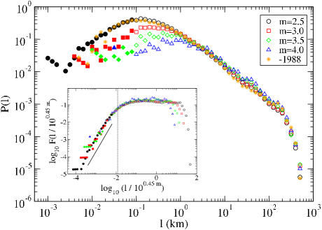
Figure 1: Distribution of distances $l$ of recurrent events for sets with different magnitude thresholds $m$. The distribution for $m=2.5$ up to 1988 is also shown. Filled symbols correspond to distances below 100 m and are unreliable due to location errors. The inset shows a data collapse, obtained by rescaling distances and distributions according to Eq. 1. The full straight line has slope 2.05; the vertical dashed line indicates the pre-factor $L_{0}$ in the scaling law for the characteristic distance, $l^{*}=L_{0}\times 10^{0.45m}$.

Fig. 1 shows the probability distribution function $P_{m}(l)$ of distances, $l$, of recurrent events for different thresholds $m$. The typical or characteristic distance, $l^{*}(m)$, where the distribution peaks, increases with magnitude. For sufficiently large $l$, all distributions show a power law decay with an exponent $\approx 1.05$ up to a cutoff. This cutoff is the size of the region of Southern California that we consider.

With a suitable scaling ansatz, the different curves in Fig. 1 fall onto a universal curve, except at the cutoff, which is a man-made scale imposed on the geological system. The inset in Fig. 1 shows results of a data collapse using

$$P_{m}(l)\sim l^{-1.05}F(l/10^{0.45m})\;.$$ (1)

The scaling function $F$ has two regimes, a power-law increase with exponent $\approx 2.05$ for small arguments and a constant regime at large arguments. The transition point between the two regimes can be estimated by extrapolating them and selecting the intersection point, giving $L_{0}=0.012$km. For the characteristic distance that appears in $F$ we thus find $l^{*}\approx L_{0}\times 10^{0.45m}$. This is close to the estimated behavior of the rupture length $L_{R}\approx 0.02\times 10^{m/2}$ km given by Kagan (2002) and remarkably close to $L_{R}=\sqrt{A_{R}}\approx 0.018\times 10^{0.46\;m}$ km given by Wells and Coppersmith (1994), where $A_{R}$ is the rupture area.

The agreement between our result and that of Wells and Coppersmith (1994) suggests that the characteristic length scale of distances of recurrent events is the rupture length, defined in terms of the rupture area $l^{*}=L_{R}\equiv\sqrt{A_{R}}$. This is substantially supported by the remarkable fact that, for fixed $m$, $P_{m}(l)$ and thus $l^{*}$ does not significantly vary with the length of the observation period despite huge differences in the number of earthquakes $N$ — which is very different from a random process (Davidsen et al., 2006). As Fig. 1 shows, $P_{2.5}(l)$ is largely unaltered if only the sub-catalog up to 1988 is analyzed. This is not true for sub-catalogs of similar size generated by randomly deleting events. The comparison of the two different observation periods in Fig. 1 further shows that $l^{*}$ does not depend strongly on the total number of recurrences (or links) or on the average degree of the network, $\langle k\rangle={\rm\#links/\#nodes}$ ($\langle k\rangle=6.56$ (7.40) for events up to 1988 (2002) and $m=2.5$), but clearly on $m$. The independence of the time span and consequent number of events implies that Eq. (1) is a robust, empirical result for seismicity.

The identification $l^{*}=L_{R}$ is also consistent with the fact that the description of earthquakes as a point process breaks down at the rupture length. Below that scale, the relevant distance(s) between earthquakes is not given solely by their epicenters but also by the relative location and orientation of the spatially extended ruptures. Due to different orientations we expect randomness or lack of correlations between epicenters for distances below the rupture length. If events are happening randomly in space, or are recorded as happening randomly in space due to location errors, then $P_{m}(l)$ rises linearly. To see this consider a two dimensional disc of radius $R$, with one point at the center and $N_{R}$ randomly distributed points. The probability that there will be no (other) point within a distance $l$ of the center point is $(1-l^{2}/R^{2})^{N_{R}}$; therefore, the probability density for the closest point to be at distance $l$ is $(2N_{R}l/R^{2})(1-l^{2}/R^{2})^{N_{R}-1}$. At small $l$, this will describe the distribution shown in Fig. 1 and determine the scaling function $F$ in Eq. (1). In fact, this is precisely what the earthquake data show for distances smaller than the rupture length (see the straight line with a slope of 2.05 in the inset of Fig. 1 and the linear increase with slope 1 in the main part of Fig. 1).

The lengths $l^{*}$ observed for the values of $m$ we consider are larger than the length ($\approx 100m$) at which we observe random behavior due to location errors. In fact, the data do not show any anomaly near $100m$. Moreover, $P_{4}(l)$ (blue triangles) does not change substantially if the epicenters in the catalog are randomly relocated by a small distance up to one kilometer. Yet, the maximum for $P_{2.5}(l)$ shifts to larger $l$ with this procedure, destroying the scaling of $l^{*}(m)$. Since the smallest $l^{*}$ that obeys the data collapse is $\approx 160$ m, the data collapse we observe for the original data verifies that the relative location errors are indeed less than $100m$, or of that order. Furthermore, our observations indicate that spatial correlations between epicenters are already lost for distances $100{\rm m}<l<l^{*}$, although the frequency of pairs of recurrent events with these small distances is much higher than by random chance (Davidsen et al., 2006).

Related to the distribution of distances of recurrent events is the distribution of distance ratios $l_{i}/l_{i-1}$ in the cascade of recurrences to a given event. Here recurrences are ordered by time; recurrence $i$ comes after $i-1$. We take $l_{0}=448.5$ km, which is the size of the region covered by the catalog (Fig. 2a). By construction these ratios are always $\leq 1$. We denote by $P_{i}(x)$ the probability density that $l_{i}/l_{i-1}=x$ for each event that has an $i^{th}$ recurrence. The data for $i=1$ (black circles) scale over a wide region as $P_{1}(x)\sim x^{-\delta_{r}}$ with $\delta_{r}\approx 0.6$ – as already shown in (Davidsen and Paczuski, 2005). This is indicated in Fig. 2a by the straight line. Although each distribution $P_{i}(x)$ is different, the curves for $i\geq 2$ also show (more restricted) power law decay comparable to $P_{1}$. For $l_{i+1}/l_{i}\to 1$ they also show a peak, which becomes more pronounced with increasing $i$. This is due to recurrences occurring at almost the same distance. The observed exponent $\delta_{r}$ for the power law decay has a dynamical origin and is not determined by the spatial distribution of seismicity (Davidsen and Paczuski, 2005): Purely based on the correlation dimension $D_{2}$, one would expect $P_{1}(x)\sim x^{D_{2}-1}$. For Southern California, this gives a growing dependence $P_{1}(x)\sim x^{0.2}$ rather than a decaying behavior. Thus, the exponent $\delta_{r}$ reflects the complex spatiotemporal organization of seismicity.

A similar analysis can be made for the distribution of recurrence times, $P_{m}(T)$ for different threshold magnitudes $m$, which is shown in Fig. 3. These distributions all decay roughly as $1/T^{\alpha}$ with $\alpha\approx 0.9$ for intermediate times as indicated in the inset. The apparent scaling region in Fig. 3 shows some curvature, though. Surprisingly, $P_{m}(T)$ is independent of $m$ and the number of events in the considered catalog. This is very different from earlier results for waiting time distributions between subsequent earthquakes (Bak et al., 2002; Corral, 2003) and reflects a new non-trivial feature of the spatiotemporal dynamics of seismicity that appears when events other than the immediately subsequent ones are considered.

The relative times between subsequent recurrences in the hierarchy can be analyzed in the same way as distances were above. Fig. 2 shows distributions of ratios of the times $T_{i}/T_{i+1}$ for subsequent recurrences to a given event. The broadest scaling regime materializes for $T_{1}/T_{2}$, again with exponent $\delta_{T}\approx 0.6$. The distributions for larger $i$ follow roughly the same behavior for ratios $\ll 1$, but deviate (less strongly than for the spatial data in Fig. 2a) when the ratios tend to 1. Again it is obvious that this behavior cannot be explained by random events.

The description of seismicity as a network of earthquake recurrences allows its characterization by means of the usual characteristics that are thought to be important for complex networks (Albert and Barabási, 2002). One such network property is its degree distribution. Fig. 2b shows the degree distributions for $m=2.5$, which is compared to a a Poisson distribution with the same mean degree $\langle k\rangle=7.40$ (solid line). A Poisson degree distribution would be expected if earthquakes epicenters were placed randomly in space and time. While the in-degree distribution agrees with such a random network, the out-degree distribution shows significant deviations. In particular, the network keeps a preponderance of nodes with small out-degree as well as an excess of nodes with large out-degree compared to a Poisson distribution. This effect is independent of magnitude, as an analysis of subsets with higher magnitude threshold shows. Note, however, that $\langle k\rangle$ decreases with $m$, simply because the catalog size shrinks with $m$. In particular, we find $\langle k\rangle=6.24,5.20,4.35$ for $m=3.0,3.5,4.0$, respectively. The non-trivial behavior of the out-degree distribution implies in particular that the network topology and, thus, the hierarchial cascade of recurrences or records captures important information about the spatiotemporal clustering of seismicity.

4 Conclusions

Our analysis shows that the description of seismicity by means of recurrences in space-time allows us to characterize its clustering behavior using only spatiotemporal relations between events and to identify new, robust scaling laws in the pattern of seismic activity. The pairs of recurrent events form a complex network with non-trivial statistics. The method allows us to detect the rupture length and its scaling with magnitude directly from earthquake catalogs without making any assumptions. Our results for the distributions of relative separations for the next recurrence in space and time should also have implications for seismic hazard assessment. Finally, our findings provide detailed, benchmark tests for models of seismicity.

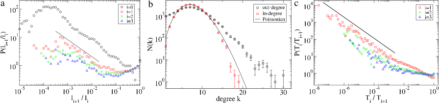
Figure 2: (a) Distribution of recurrence distance ratios $l_{i+1}/l_{i}$. The straight line corresponds to a decay with exponent 0.6. (b) Distributions of in- and out-degrees of the network for $m=2.5$. The given error bars correspond to $\sqrt{N(k)}$. (c) Distribution of recurrence time ratios $T_{i}/T_{i+1}$. The straight line has slope -0.62.

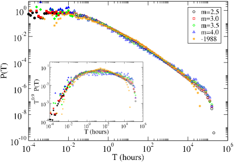
Figure 3: Distributions of recurrence times for different threshold magnitudes $m$. The distribution for $m=2.5$ up to 1988 is also shown. Filled symbols correspond to times below 90 seconds which are underestimated and unreliable due to measurement restrictions. The inset shows the rescaled distributions.