The bulk of the stock market correlation matrix is not pure noise

Abstract

We analyse the structure of the distribution of eigenvalues of the stock market correlation matrix with increasing length of the time series representing the price changes. We use 100 highly-capitalized stocks from the American market and relate result to the corresponding ensemble of Wishart random matrices. It turns out that systematically more eigenvalues stay beyond the borders prescribed by this variant of the Random Matrix Theory (RMT). This may indicate that even the bulk of the spectrum of the stock market correlation matrix carries some sort of correlations that are masked by a measurement noise when the time series used to construct the matrix are short. We also study some other characteristics of the ”noisy” eigensignals, like their return distributions, temporal correlations or their multifractal spectra and the results support the above conclusions.

1 Introduction

The formalism of correlation matrix is widely used in contemporary finance both on theoretical and on practical level in order to estimate correlation structure of a financial market or in order to create portfolios characterized by given properties. This formalism is especially important for various risk management techniques like e.g. the Markowitz optimal portfolio theory [1] which helps one constructing portfolios offering minimal risk at a given return or maximal return at a given risk. This theory uses eigenvalues of the correlation matrix as a measure of the portfolio’s risk: no matter which eigenvalue one uses, it is fully informative and a corresponding portfolio is therefore valid. However, recently such understanding of the portfolio selection has been strongly challenged in a series of papers linking the correlation matrix formalism and the portfolio theories with Random Matrix Theory (RMT) and the ensemble of Wishart matrices (sample random correlation matrices) in particular [2, 3]. Accordingly, the current view is that only a few eigenvalues and eigenvectors of the correlation matrix are important in practice and carry any significant information about the market, while all others describe nothing more than pure noise. Thus, only those few portfolios which correspond to the non-random eigenstates of the correlation matrix can be in fact regarded as a potential investment target. This observation profoundly restricting the applicability of classical portfolio theories rises a question of how to reconcile the two contradicting views on the RMT-like portfolios. This problem is at present one of central issues of econophysics and is intensively studied by many different groups. One of directions in which current analyses go is the so-called denoising of the correlation matrices which aims at removing the estimation errors of the correlations due to finite size of empirical data [4, 5, 6, 7]. Another possible approach is to look into the empirical data and to answer the question what is there really random and what is not. In order to do this, one can firstly investigate the properties of dynamics of different portfolios calculated by using the correlation matrix framework, to compare characteristics of random and non-random ones, and, possibly, to identify those signatures of the dynamics which represent some non-random phenomena even in the case of the RMT-like eigenstates. In the present paper we would like to follow this idea and draw some conclusions based on data from the American stock market.

2 Formalism

In general, a portfolio $P$ consists of a number of securities $X_{s},s=1,...,N$ associated with weights $w_{s}$ characterizing the fraction of total amount of capital invested in a particular security. Return of such a portfolio after time $\Delta t$ is the weighted sum of logarithmic price increments $g_{s}(\Delta t)=\ln p_{s}(t+\Delta t)-\ln p_{s}(t)$ of individual securities $X_{s}$:

$$G_{P}(\Delta t)=\sum_{s=1}^{N}w_{s}g_{s}(\Delta t).$$ (1)

By fixing the time scale $\Delta t$ and creating a time series of length $T$ from consecutive discrete-time portfolio’s returns $\{G_{P}(j)\}_{j=1}^{T}$ it is also possible to investigate dynamics of the portfolio in time. Although every possible set of weights define certain portfolio, from an investor’s perspective only those portfolios which are characterized by specific predefined properties can be of practical interest. For example, a portfolio which is least risky among family of ones offering the given future return $G_{P}$. Risk $R(P)$ is usually quantified in terms of variance of the time series of historical returns

$$R(P)=\sigma^{2}(P)={\rm var}\{G_{P}(j)\}_{j=1}^{T}.$$ (2)

According to the classical Markowitz theory, this risk can be related to correlations (or covariances) between the time series of individual security returns $g_{s}(j),j=1,...,T$ for the relevant group of securities.

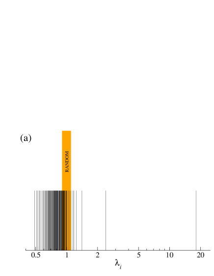
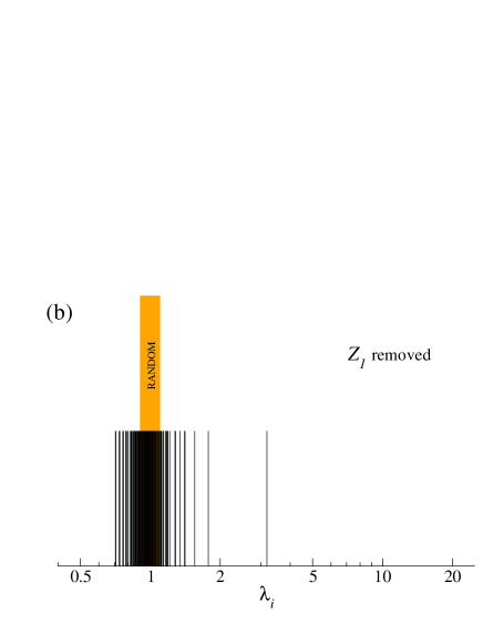
Figure 1: Empirical eigenvalue spectrum of the correlation matrix ${\bf C}$ (vertical lines), calculated for 100 highly capitalized American companies over the period 1998-1999; the eigenvalues of a random Wishart matrix with the same $Q$ may lie only within the shaded vertical region (a). Eigenvalue spectrum after effective rank reduction of ${\bf C}$, i.e. after subtracting the contribution of the most collective eigensignal $Z_{1}$ (b) and the two most collective ones $Z_{1}$ and $Z_{2}$ (c).

More specifically, let one consider a set of $N$ securities (e.g. stocks) each represented by a time series of normalized returns $g_{s}(j),s=1,...,N;j=1,...,T$. From these time series an $N\times T$ data matrix ${\bf M}$ can be created and then a correlation matrix ${\bf C}$ according to the formula

$${\bf C}=(1/T){\bf M}{\bf M}^{\rm T}.$$ (3)

Each element of ${\bf C}$ is obviously the Pearson correlation coefficient $C_{m,n}$ between a pair of signals $m$ and $n$. The correlation matrix can be diagonalized by solving the eigenvalue problem

$${\bf C}{\bf x}_{i}=\lambda_{i}{\bf x}_{i},\ \ i=1,...,N.$$ (4)

From the point of view of investment theories, each eigenvector ${\bf x}_{i}$ can be considered as a realization of an $N$-security portfolio $P_{i}$ with the weights equal to the eigenvector components $x_{i}^{(k)},k=1,...,N$. For a non-degenerate matrix ${\bf C}$, $P_{i}$ and $P_{j}$ are independent for each pair of their indices, which allows one to choose such a portfolio, whose risk is independent of others.

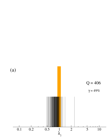
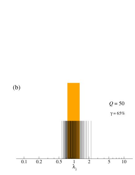
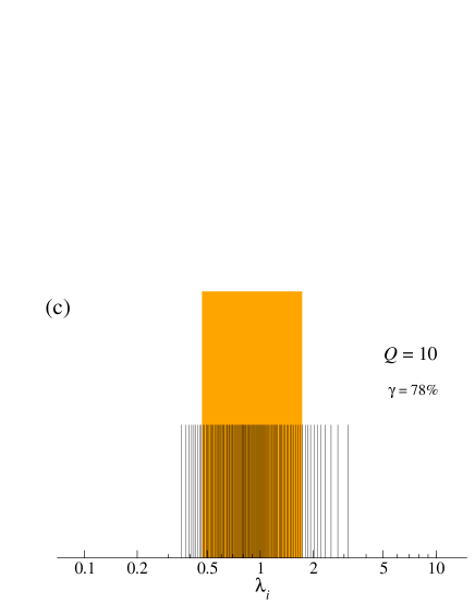
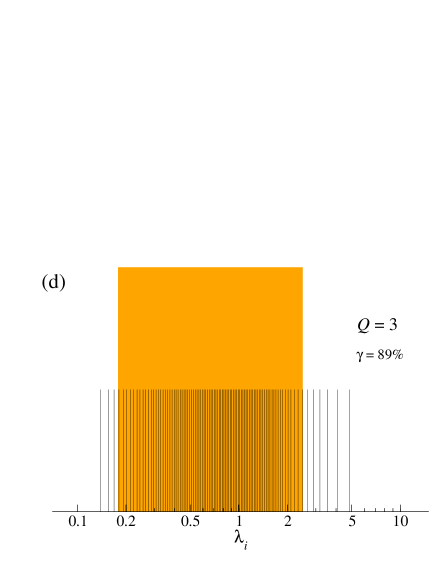
Figure 2: Empirical eigenvalue spectrum of correlation matrix ${\bf C^{\prime}}$ (see text) after subtracting the contribution of the two most collective components associated with $\lambda_{1}$ and $\lambda_{2}$ for four different values of $Q$; (a) is the same as Fig. 1(c). Shaded regions correspond to RMT predictions for given $Q$.

From a dynamical perspective, each eigenvector (and thus portfolio) can be associated with the corresponding time series of the portfolio’s returns by the expression analogous to Eq.(1)

$$z_{i}(j)=\sum_{k=1}^{N}x_{i}^{(k)}g_{k}(j),\ \ i=1,...,N;\ j=1,...,T.$$ (5)

These time series we shall call the eigensignals $Z_{i}$ (see also [8, 9] for an alternative realization). One of the most important properties of such eigensignals is that their risk can be easily related with the corresponding eigenvalues:

$$R(P_{i})=\sigma^{2}(Z_{i})={\bf x}_{i}^{\rm T}{\bf C}{\bf x}_{i}=\lambda_{i},$$ (6)

Thus, the eigenvalue size is a risk measure and, in consequence, the larger $\lambda_{i}$, the larger variance of $Z_{i}$ and also the larger risk of the corresponding portfolio $P_{i}$.

3 Results

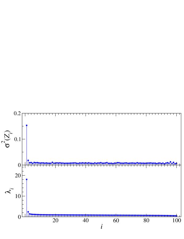
Figure 3: Standard deviation $\sigma(Z_{i})$ for all eigensignals $Z_{i}$ (top panel) together with the corresponding eigenvalues $\lambda_{i}$ (bottom panel). Almost perfect correspondence between both panels is visible; the difference in units in the vertical axes is due to eigenvector normalization performed by diagonalization procedure.

We analyzed high-frequency data from the American stock market [10] in the period 1 Dec 1997 $-$ 31 Dec 1999. In order to calculate inter-stock correlations we chose a set of stocks of $N=100$ highly capitalized companies listed in NYSE or NASDAQ (capitalization $>\$10^{10}$ in each case). These stocks are frequently traded (0.01-1 transactions/s) and hence the time scale of $\Delta t=5$ min allowed us to perform a statistically significant analysis; such a short time scale was also desired because of length of time series (approx. 40,000 data points). Typically, the portfolio analysis is performed on daily data; usually this time scale is recommended because of the fact that at this scale the correlations present at the market are well-developed. However, restricting the analysis to such long $\Delta t$ seems not to be necessary in contemporary markets, in which both pieces of information arrive more frequently and the investors react to them quicker than in the past. This obviously leads to acceleration of the market time paced by consecutive transactions. Thus, as recent papers document [13, 14], for highly capitalized stocks which are also among the most frequently traded ones, the correlations reach their saturation level at the time horizons much shorter than a day. In case of our data this time horizon corresponds to about 30 min, while for $\Delta t=5$ min the correlations associated with $\lambda_{1}$ are clearly very pronounced and informative and $\lambda_{1}$ assumes approx. 2/3 of its saturation level [14].

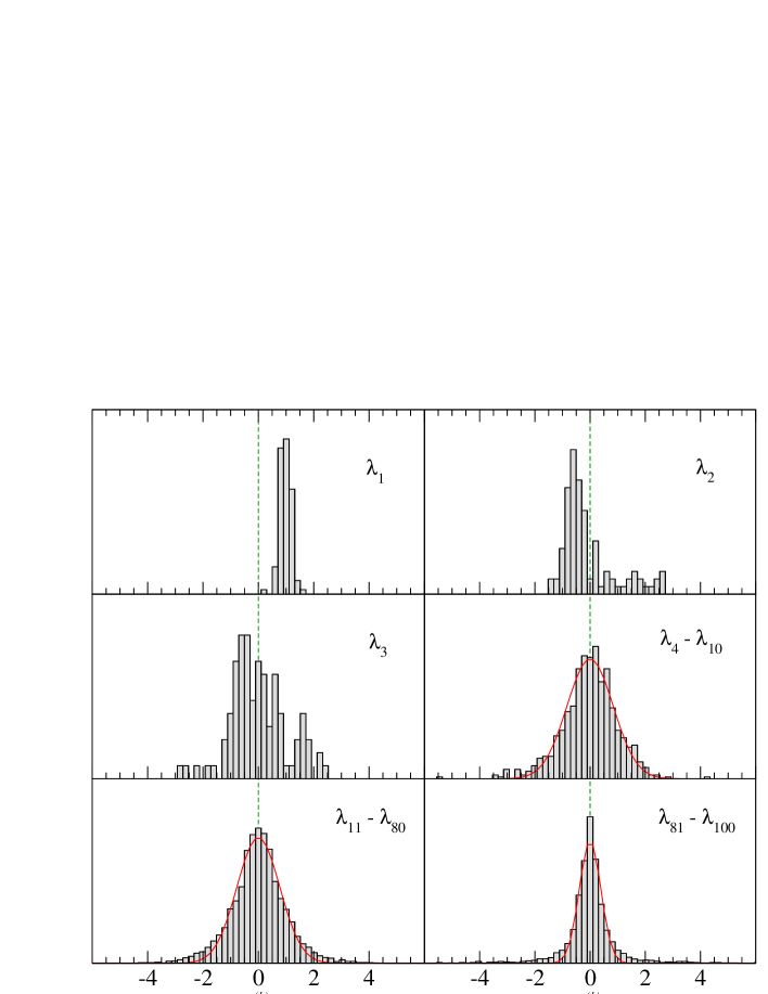
Figure 4: Histograms of eigenvector components $x_{i}^{(k)}$ for different eigenvalues $\lambda_{i}$. A Gaussian is fitted to the empirical histograms corresponding to the most random eigenvectors.

3.1 Eigenvalue distribution

The eigenvalue distribution offers a representative and the most frequently used measure to quantify the characteristics of matrices, especially in the context of relating them to RMT. Let us therefore start presentation of the results with the eigenvalue spectrum of the correlation matrix. Figure 1(a) shows all 100 eigenvalues distributed along the horizontal axis, denoted by vertical lines. The largest eigenvalue $\lambda_{1}\simeq 18$, repelled from the rest of the spectrum, describes the collective eigenstate which can be identified with the market. $\lambda_{2}\simeq 2.4$ absorbs some collectivity either, but its magnitude is by an order of magnitude smaller than $\lambda_{1}$ and can be related with some branch-specific factor (the same applies to a few next eigenvalues). Figure 1(a) displays that only a small fraction of $\lambda_{i}$’s falls within the RMT region defined by its bounds: $\lambda_{\rm min}^{\rm max}=1+1/Q\pm 2/\sqrt{Q}$ (shaded vertical region in Figure), where $Q=T/N\simeq 406$ [15]. However, due to the fact that ${\rm Tr}{\bf C}=100$, the existence of strong collective components can effectively supress the noisy part of the ${\bf C}$ eigenspectrum, shifting smaller eigenvalues towards zero. Therefore, in order to correct for this effects it is recommended to remove the market factor $Z_{1}$ from the data [11]. This can be done by means of the least square fitting of this factor represented by $z_{1}(j)$ to each of the original stock signals $g_{k}(j)$:

$$g_{k}(j)=\alpha_{k}+\beta_{k}z_{1}(j)+\epsilon_{k}^{(1)}(j),$$ (7)

where $\alpha_{i},\beta_{i}$ are parameters, and then we can construct a new correlation matrix ${\bf C}^{(1)}$ from the residuals $\epsilon_{k}^{(1)}(j)$ (e.g. ref. [2, 11]). Now significantly more eigenvalues fall within the shaded RMT region as Figure 1(b) documents. This can be done once again and the $\lambda_{2}$ component can also be removed leading to the eigenspectrum presented in Figure 1(c). In fact, now many more eigenvalues ($\gamma=49$%) overlap with the RMT interval $<\lambda_{\rm min},\lambda_{\rm max}>$, though, interestingly, this value is qualitatively different from results presented earlier in [2, 11, 8] where vast majority of the eigenvalues was inside the RMT bounds.

In order to shed some light on this problem we note that in both cited works the parameter $Q$ was much smaller than in our case: $Q=4.1$ and 6.4 in ref. [11] and $Q=3.2$ in [2] and therefore the RMT spectrum was respectively wider. By manipulating the $Q$ value for our data (we divide the time series into windows of length $T^{\prime}$ with predefined $Q^{\prime}=T^{\prime}/N$, then we calculate ${\bf C}^{\prime}$ for each window and average its eigenspectrum over all the windows) we obtain the correlation matrix eigenspectrum which can be compared with the original one for the undivided time series ($Q=406$). Since in each case the average $\lambda_{1}$ is strongly repelled (and its value is approximately the same as in Fig. 1(a)), we follow the earlier procedure and remove the collective components related to both $\lambda_{1}$ and $\lambda_{2}$ for each window before averaging the resulting eigenspectra. Figure 2 shows such decollectified average eigenspectra for four different values of $Q$. What is immediately evident, the wider the shaded RMT region, the more eigenvalues it overlaps with. For the smallest presented $Q=3$ as much as $\gamma=89$% eigenvalues fall within the RMT realm which is compatible with $\gamma=94$% from ref. [2]. Naturally, as we verified by an explicit calculation, this observation obtained for $\Delta t=5$ min qualitatively remains unaltered if we pass to longer time scales e.g. $\Delta t=60$ min, despite the fact that the corresponding time series shorten and the maximum available $Q$ decreases. We conclude that for a typical realization of $Q<10$ in practical applications (usually large $N$ and relatively small $T$ as it happens for daily data), only the largest eigenvalues are able to deviate from the RMT predictions, while the other eigenvalues possibly carrying some more subtle correlations may be forced to spuriously merge with the random bulk. This purely statistical effect suggests that the random part of the ${\bf C}$ eigenspectrum can in fact comprise non-random components which can be discerned from noise only if one uses data with larger $Q$. This is in favour of using data also with frequencies higher than the daily one as a tool for denoising ${\bf C}$. (It is noteworthy that a parrallel effect of shifting the small non-random eigenvalues ($\lambda_{i}\approx\lambda_{\rm min}$) into the RMT interval has been presented recently in ref. [12].)

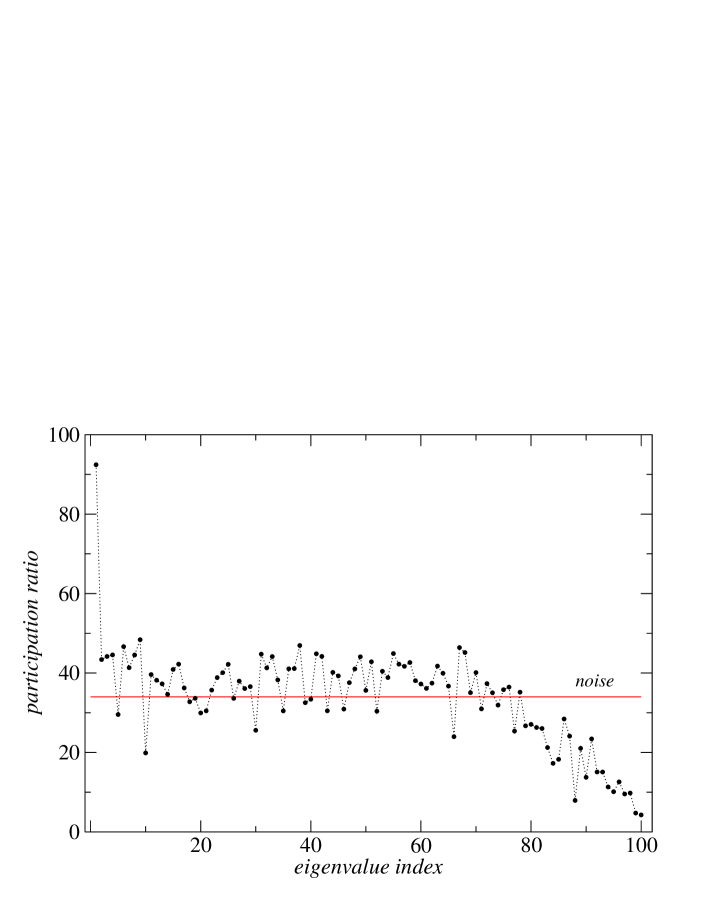
Figure 5: Reciprocal of inverse participation ratio (Eq.(8)) for all 100 eigenvectors of the correlation matrix. Noise level for random Gaussian case is also presented.

3.2 Eigenvector properties

Figure 3 illustrating the strong relation between the risk and the eigenvalues (Eq.(6)), displays the eigensignal variance calculated for each $Z_{i}$ (upper panel) and all the eigenvalues of ${\bf C}$ (lower panel). Essentially no significant qualitative difference between these two quantities can be found, exactly as expected. Apart from the eigenvalue spectrum, RMT offers useful predictions regarding distribution of the eigenvector components for a completely random matrix, which assumes the form of the Porter-Thomas (Gaussian) distribution. In contrast, in the case of a collective non-random eigenvector, there exists some kind of vector localization or delocalization. Figure 4 presents distributions of the components for typical eigenvectors of our matrix and for a few specific cases. The eigenvector corresponding to the largest eigenvalue $\lambda_{1}$ is completely delocalized because all its components are roughly the same and the associated distribution is centered at 0.1. This is standard situation and in evolution of the stock prices this eigenvector represents the market factor. Also non-random is the eigenvector for $\lambda_{2}$ with the components distribution still far from Gaussian. A trace of randomness however occurs already for $\lambda_{3}$ and is clear for a bulk of eigenvectors in the next panel of Figure 4. On the other hand, for the extremely small eigenvalues, localization can be perfectly seen.

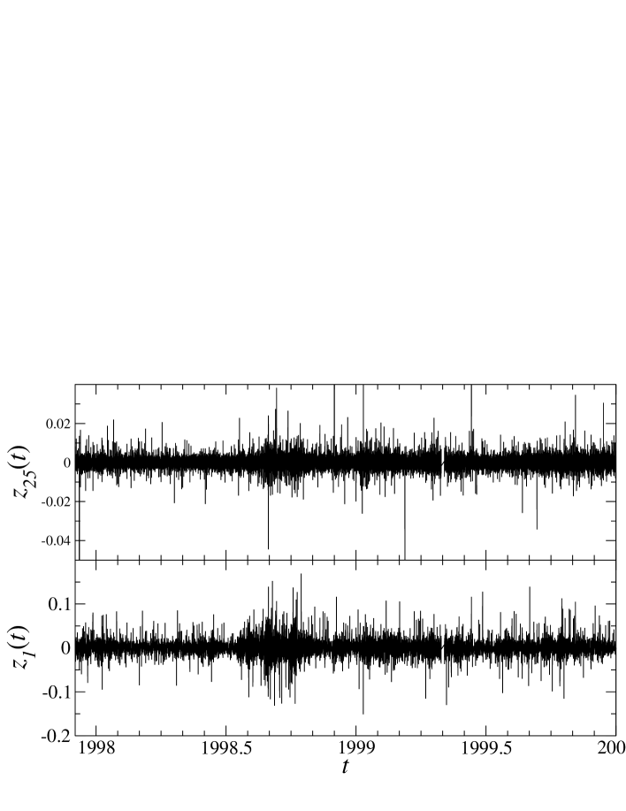
Figure 6: Time series of the eigensignals for $\lambda_{1}$ (top) and $\lambda_{25}$ (bottom). Note different scales in vertical axes of both panels.

One of the key properties of the eigenvector (and thus also the eigenstate $Z_{i}$) is the effective number of its large components. A related measure is inverse participation ratio

$$I_{i}=\sum_{k=1}^{N}(x_{i}^{(k)})^{4},\hskip 14.22636ptk=1,...,N$$ (8)

and its reciprocal $1/I_{i}$ (“participation ratio”). Figure 5 presents this latter quantity calculated for all the eigenvectors together with its value $N/3$ for random case in which $x_{i}^{(k)}$ are taken independently from normal distribution. For $i=1$ almost all the companies contribute to the corresponding eigenvector $Z_{1}$, which justifies treating this eigenvector as the market factor. The eigenvectors for a few smaller eigenvalues show also slightly higher number of participating companies than for the random case but, in contrast, the eigensignals associated with the smallest 20 eigenvalues allow one to characterize them as the components related to only few stocks. The rest of the eigenvectors seem to be random, with small deviation from the predicted value of $N/3$ probably due to the existence of fat tails of the returns distributions.

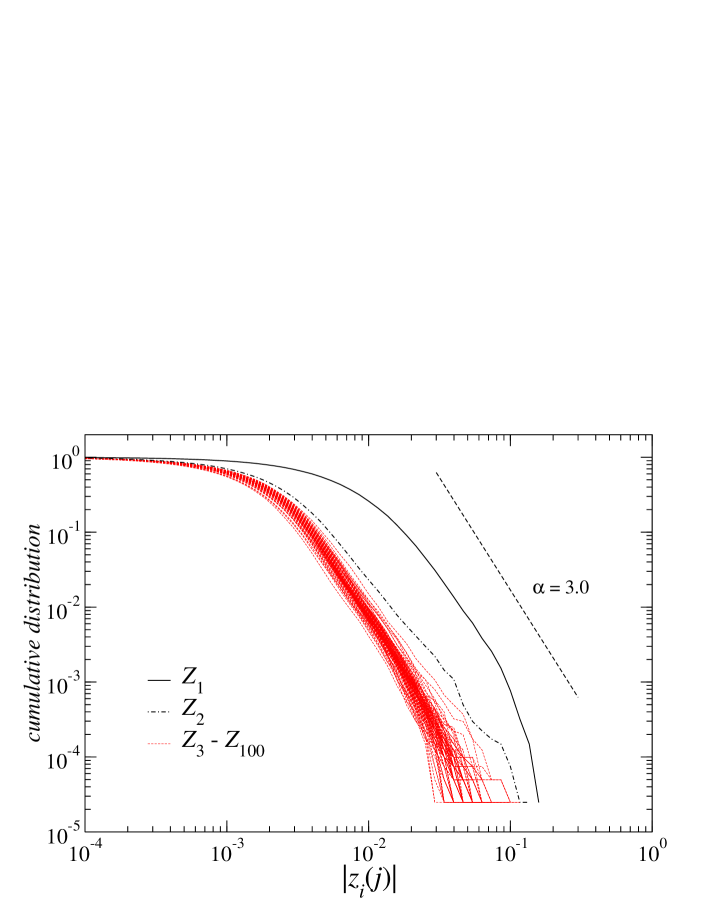
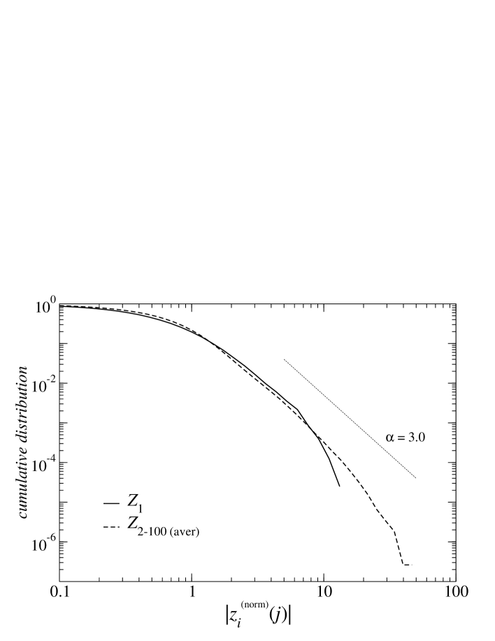
Figure 7: (a) Cumulative distribution functions for the eigensignal returns for all $Z_{i}$ ($i=1,...,N$). Distributions for $Z_{1}$ (thick solid) and $Z_{2}$ (dot-dashed) are distinguished. Inverse cubic power law ($\alpha=3.0$) is also denoted by dashed line. (b) The c.d.f. for the eigensignal returns after normalization to unit variance and averaging over $Z_{i},i=2,...,100$ (dashed) together with c.d.f. for $Z_{1}$ (solid).

Figure 6 presents the time series of the eigensignal returns $z_{1}(j)$ calculated according to Eq.(5) for $\lambda_{1}$ and $\lambda_{25}$. Curiously, if one compares both series visually, forgetting the difference in vertical axis, it could be quite difficult to point out which of the two corresponds to the most collective eigenstate. Both eigensignals are nonstationary with likely extreme fluctuations and both of them reveal also volatility clustering. Thus, one can infer that there are statistical properties which are invariant under change of the eigenstates with only minor differences between collective and noisy eigenstates.

In agreement with Figure 3, c.d.f. of the eigensignal returns (Figure 7(a)) show that $Z_{1}$ is characterized by much broader distribution than other eigensignals, and that the same, but to a lesser extent, is true also for $Z_{2}$. It is interesting that, except for $Z_{1}$, all the eigensignals are associated with the distributions with the power law scaling in tails, almost exactly like for the original stock returns (see e.g. [13, 16, 17, 18]). Only $Z_{1}$ presents different behaviour: a short range of power law scaling and significant deviation from this behaviour for $|z_{1}|>5\sigma$. This can be even more convincing if all the signals are normalized to unit variance (Figure 7(b)); the power law slope with $\alpha\simeq 3$ is typical for all the eigensignals (although for a considerably larger $\Delta t$ exactly this kind of scaling may not be observed [13], the eigensignal c.d.f.s also preserve tails of the individual stock returns c.d.f.s for the same $\Delta t$). The non-typical shape of c.d.f. for $Z_{1}$ in Figure 7(b) can originate from the fact that this eigensignal is composed as an average of almost 100 individual stocks, while on average 1/3 of this number of stocks contribute to other eigensignals; this is why Central Limit Theorem leaves its fingerprints presumably on $Z_{1}$. However, this cannot be considered as a rule, because for significantly larger time scales (e.g. $\Delta t=60$ min) or for some other groups of stocks for which the cross-correlations are more intensive such a peculiarity of the $Z_{1}$’s c.d.f. might not be observed. Noteworthy to mention is that the inter-stock correlations responsible for a transfer of scaling [17] from the stock returns to the eigensignal distributions in Figure 7 are mainly linear (thus detectable by the correlation matrix). However, the very fact that scaling exists at $\Delta t=5$ min or at longer time scales is an effect of highly nonlinear temporal correlations present in the stock returns (the volatility autocorrelations etc.) which may also be detectable in the eigensignals (see the next subsection).

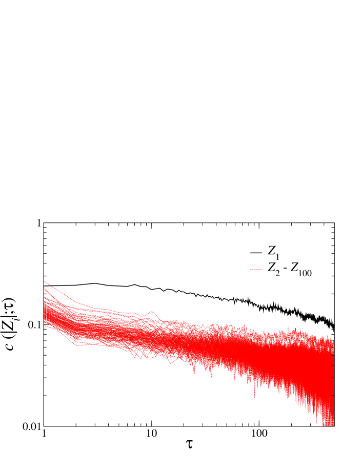
Figure 8: Volatility autocorrelation function $C(|Z_{i}|,\tau)$ for $i=1,...,100$. For each eigensignal $Z_{i}$, daily trend was removed by the standard detrending procedure (see [31, 32]).

3.3 Temporal correlations

Now let us look at temporal correlation properties of the eigensignals. Figure 8 shows the volatility autocorrelation function $c(|Z_{i}|;\tau)\equiv c(|z_{i}(j)|,|z_{i}(j+\tau)|)$ for all the eigensignals $Z_{i}$. The difference between $Z_{1}$ and the rest of signals is pronounced and resembles the corresponding difference in the case of the eigensignals variance (Figure 3). In fact, memory in $Z_{1}$ is about two orders of magnitude longer than for the other eigensignals (for $m>1$: $c(|Z_{i}|;\tau)\simeq c(|Z_{1}|;10^{2}*\tau)$). However, it cannot be said that $Z_{1}$ (the market component) absorbs all the memory of the evolution of stock prices. The volatility autocorrelation function for the other eigensignals decay very slowly in time as well.

Another interesting sort of nonlinear correlations are cross-correlations between returns and volatility $c(Z_{i},|Z_{i}|;\tau)$. It has been observed that past returns imply negatively correlated future moves in volatility, the so-called leverage effect [19, 20, 21]. Figure 9 shows the cross-correlation function $c(Z_{i},|Z_{i}|;\tau)$ for the returns and the volatility for all the eigensignals. The leverage effect can be detected easily only for $i=1,2,3$; all other eigensignals do not reveal it. For $i=1$ and $i=2$ the correlations are qualitatively the same despite the earlier-presented differences between the eigensignals. For $i=3$ negative correlations do not exist for the smallest values of $\tau$, while they are the strongest for $\tau>100$. In order to carry out this calculation we took signals for $\Delta t=20$ min, because analogous signals at smaller time scales are too noisy to show the strong leverage effect. Interestingly, for the original signals $g_{s}$ corresponding to individual stocks $s$, the leverage effect is much weaker and even difficult to observe at all.

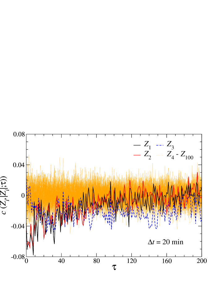
Figure 9: Cross-correlation function $c(Z_{i},|Z_{i}|;\tau)$ for time series of returns $Z_{i}$ and of volatility $|Z_{i}|$ calculated for all eigensignals separately. The resulting functions for the eigensignals corresponding to three largest eigenvalues are distinguished by thick lines.

3.4 Multifractal characteristics

One of the consequences of the broad probability distributions (Figure 7) and of the nonlinear correlations (Figure 8 and 9) is multifractal character of signals, i.e. the existence of a continuous spectrum of scaling indices $f(\alpha)$. It has already been shown in numerous works that stock returns form signals which are multifractal both on daily and on high-frequency time scales [22, 23, 24, 25, 26, 27, 28, 29, 30, 32]. This behaviour can be even modeled with a good agreement if one introduces statistical processes based on multiplicative cascades [21, 33, 34, 35, 36]. Due to the fact that, by definition, the eigensignals are calculated as a sum of stock returns, the multifractality of their components can be transferred to the resulting eigensignal. Therefore one can expect that at least some of $Z_{i}$’s are also multifractal; there can exist differences in their singularity spectra because of different stock compositions for different $i$’s, though. Owing to superiority of Multifractal Detrended Fluctuation Analysis (MFDFA) [37] over Wavelet Transform Modulus Maxima (WTMM) method [38] in the case of financial data [39], we applied former one to our time series in order to calculate the singularity spectra $f(\alpha)$.

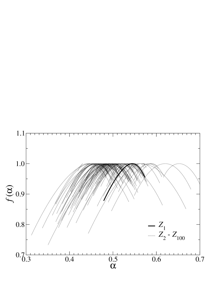
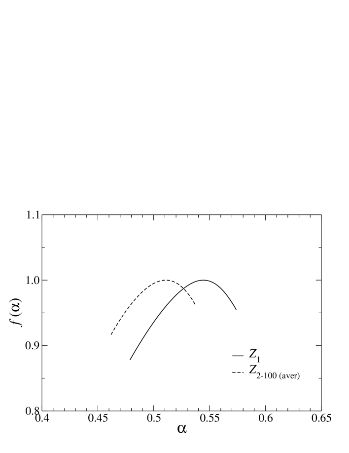
Figure 10: (a) Singularity spectra $f(\alpha)$ for eigensignals corresponding to all correlation matrix eigenvalues $\lambda_{i}$. Spectrum for the eigensignal $Z_{1}$ associated with the largest eigenvalue is denoted by a thick solid line; (b) singularity spectrum for $Z_{1}$ (solid) compared with the average spectrum for all other eigensignals $Z_{i},\ i=2,...,100$ (dashed).

We start from our eigensignal $i$ represented by the time series $z_{i}(j)$ of length $N_{es}$ and estimate the signal profile

$$Y(j)=\sum_{k=1}^{j}{(z_{i}(k)-<z_{i}>)},\ j=1,...,N_{es}$$ (9)

where $<...>$ denotes averaging over $z_{i}(k)$. In the next step $Y$ is divided into $M_{es}$ segments of length $n$ ($n<N_{es}$) starting from both the beginning and the end of the time series so that eventually there are $2M_{es}$ segments. In each segment $\nu$ we fit a $l$-th order polynomial $P_{\nu}^{(l)}$ to the data, thus removing a local trend. Then, after calculating the variance

$$F^{2}(\nu,n)=\frac{1}{n}\sum_{k=1}^{n}\{Y[(\nu-1)n+k]-P_{\nu}^{(l)}(k)\}^{2}$$ (10)

and averaging it over $\nu$’s, we get the $q$th order fluctuation function

$$F_{q}(n)=\bigg{\{}\frac{1}{2M_{es}}\sum_{\nu=1}^{2M_{es}}[F^{2}(\nu,n)]^{q/2}\bigg{\}}^{1/q},\ \ q\in\mathbf{R}$$ (11)

for all values of $n$. The most important property of $F_{q}(n)$ is that for a signal of the fractal character it obeys a power-law functional dependence on $n$:

$$F_{q}(n)\sim n^{h(q)},$$ (12)

at least for some range of $n$. As a result of complete MF-DFA procedure we obtain a family of generalized Hurst exponents $h(q)$, which form a decreasing function of $q$ for a multifractal signal or are independent of $q$ for a monofractal one. A more convenient way to present the fractal character of data graphically is to calculate the singularity spectrum $f(\alpha)$ by using the following relations:

$$\alpha=h(q)+qh^{\prime}(q)\hskip 28.45274ptf(\alpha)=q[\alpha-h(q)]+1.$$ (13)

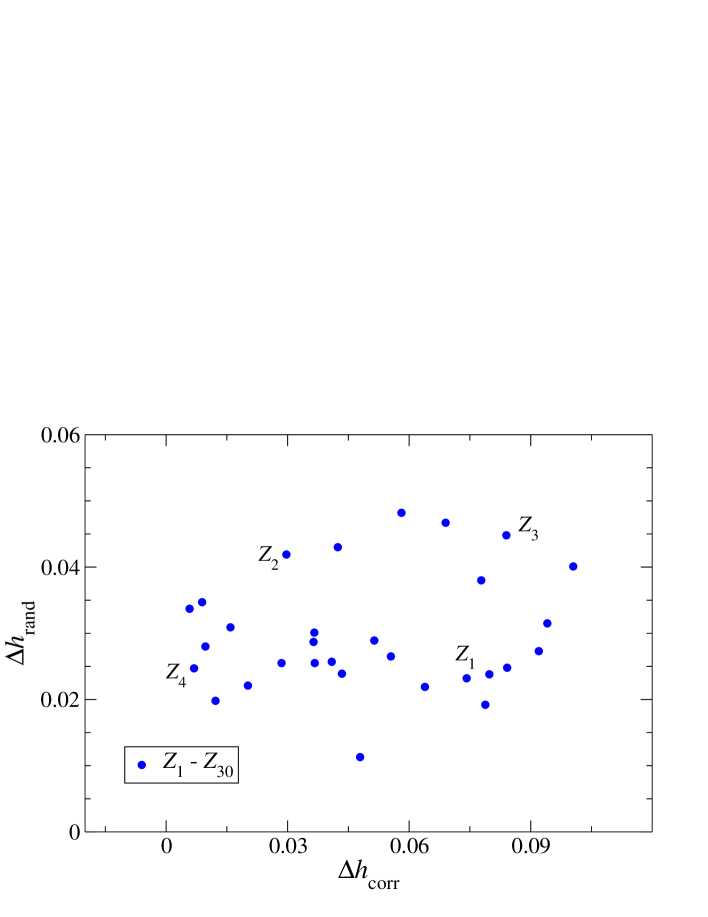
Figure 11: $\Delta h_{\rm corr}$ vs. $\Delta h_{\rm rand}$ for eigensignals corresponding to 30 largest eigenvalues. Symbols denoting $Z_{1},...,Z_{4}$ are labeled.

We computed the $f(\alpha)$ spectra with MF-DFA for all time series $Z_{i}$ and for $\Delta t=5$ min (shorter time scales are too noisy, while longer ones are represented by too short series for a reliable estimation of $f(\alpha)$) and the corresponding results are shown in Figure 10(a). Wide spectra prove that all $Z_{i}$’s are multifractal with only minor differences in widths of the spectra for different eigensignals. Although positions of maxima of the spectra vary, there is no significant $i$-dependence both in the positions and in shape of the spectra. It is interesting that even the most collective and correlated eigensignal for $\lambda_{1}$ (the solid, distinguished line in Figure 10(a)) does not develop spectrum which could deviate from the typical one. This is even more evident if we compare the spectrum for $Z_{1}$ with the average spectrum calculated from all other $Z_{i}$’s in Figure 10(b). Such similarity of multifractal properties of the eigensignals representing completely different correlation structure and different p.d.f.’s can suggest that the eigensignals corresponding to a few largest $\lambda_{i}$’s and the ones corresponding to the bulk of the eigenspectrum are in fact much more similar to each other than it is usually assumed. This also bears a serious concern regarding the justification of treating the “noisy” eigenstates as completely random without any information content.

As we already know the autocorrelations of volatility $|Z_{i}|$ for $i=1$ are different from those for $i>1$ (Figure 8), while the normalized returns have similar c.d.f.’s for all $i$. Now we would like to compare the fractal properties of different eigensignals in order to separate the two sources of multifractality: the broad distributions of returns and the correlations, and to compare the singularity spectra $f(\alpha)$ for these sources. We follow the idea of [40] and we study variability of generalized Hurst exponents $h(q)$ for the actual and the reshuffled eigensignals. If we denote the generalized Hurst exponent for the randomized signal by $h_{\rm rand}(q)$, its correlation counterpart reads

$$h_{\rm corr}(q):=h(q)-h_{\rm rand}(q).$$ (14)

Variability of $h(q)$ can be expressed by the difference

$$\Delta h:=h(q_{\rm min})-h(q_{\rm max})$$ (15)

and, analogously, the variability of $h_{\rm rand}(q)$ and $h_{\rm corr}(q)$. Each symbol in Figure 11 presents positions of the eigensignals $Z_{i}$ in ($\Delta h_{\rm corr},\Delta h_{\rm rand}$) coordinates. Eigensignals corresponding to the four largest eigenvalues are labelled. The higher value of $\Delta h_{\rm rand}$, the richer the multifractal behaviour due to the fat-tailed probability distributions of returns. Analogously, high values of $\Delta h_{\rm corr}$ indicate strong contribution of the temporal correlations. These temporal correlations implying the observed multifractal behaviour of signals have to be strongly nonlinear: our earlier calculations [32] showed that even the volatility autocorrelations that are nonlinear in returns are not capable of producing this phenomenon. Furthermore, it can be easily inferred from Figure 11 that there is nothing characteristic in the positions of the symbols related to $Z_{1,...,4}$. Results collected in Figure 10(b) and Figure 11 indicate that the multifractal analysis cannot point out any essential differences between the collective eigenstates and the noisy ones.

4 Conclusions

We analysed the eigensignals corresponding to different eigenvalues of the empirical correlation matrix calculated for the 100 highly-capitalized American companies. From a practical point of view, these eigensignals represent temporal evolution of specific portfolios defined by the corresponding eigenvectors of ${\bf C}$. We showed that despite the important differences in interpretation of different eigensignals, $Z_{i}$’s for the collective and for the noisy eigenvalues can reveal different or similar statistical properties depending on a particular quantity. What differs most is risk expressed by variance of an eigensignal, which is very high for the most collective $Z_{1}$, is also significant for $Z_{2}$, and is much smaller for the rest of the $Z_{i}$’s. This is closely related to the eigenvector properties, which are different for highest and other $\lambda_{i}$’s. The risk is also related to the width of the returns distributions, preventing the eigensignals for small eigenvalues from high fluctuations and the associated portfolios from large losses. The second group of quantities which reveal different values for different $Z_{i}$’s are nonlinear correlations, both those in volatility and those between returns and volatility. On the other hand, there are properties that remain unaltered when going from small to large values of $i$. The most interesting one is the multifractality of all eigensignals which is surprisingly roughly the same for different $Z_{i}$’s. Curiously, this happens even if the above-mentioned correlations vary among the eigensignals. One of possible sources of this can be similar shape of tails of the probability distributions, which after normalizing the eigensignal returns show the inverse cubic scaling for all $i$. Both the fat-tailed distributions of returns and the multifractal character of eigensignals for each eigenvalue lead to a conclusion that the noisy eigenstates might not be so random as they are usually regarded by their relation to RMT. Rich multifractal dynamics of the eigensignals corresponding to even the random part of the eigenvalue spectrum suggests that strong nonlinear correlations are present in the temporal evolution of each portfolio giving it significance which exceeds pure noise. This conclusion is strongly supported by the observation (Section 3.1) that many real correlations may be masked by noise due to too short signals considered in practical applications.

References

- [1] H. Markowitz, J. Finance 7 (1952) 77-91
- [2] L. Laloux, P. Cizeau, J-.P Bouchaud, M. Potters, Phys. Rev. Lett. 83 (1999) 1467-1470
- [3] V. Plerou, P. Gopikrishnan, B. Rosenow, L.A.N. Amaral, H.E. Stanley, Phys. Rev. Lett. 83 (1999) 1471-1474
- [4] S. Pafka, I. Kondor, Eur. Phys. J. B 27 (2002) 277-280
- [5] S. Pafka, I. Kondor, Physica A 319 (2003) 487-494
- [6] S. Pafka, I. Kondor, Physica A 343 (2004) 623-634
- [7] Z. Burda, J. Jurkiewicz, Physica A 344 (2004) 67-72
- [8] J. Kwapień, S. Drożdż, F. Grümmer, F. Ruf, J. Speth, Physica A 309 (2002) 171-182
- [9] J. Kwapień, S. Drożdż, A.A. Ioannides, Phys. Rev. E 62 (2000) 5557-5564
- [10] http://www.taq.com
- [11] V. Plerou, P. Gopikrishnan, B. Rosenow, L.A.N. Amaral, T. Guhr, H.E. Stanley, Physical Review E 65 (2002) 066126
- [12] A. Utsugi, K. Ino, M. Oshikawa, Phys. Rev. E 70 (2004) 026110
- [13] S. Drożdż, J. Kwapień, F. Grümmer, F. Ruf, J. Speth, Acta Phys. Pol. B 34 (2003) 4293-4306
- [14] J. Kwapień, S. Drożdż, J. Speth, Physica A 337 (2004) 231-242
- [15] A.M. Sengupta, P.P. Mitra, Phys. Rev. E 60 (1999) 3389-3392
- [16] V. Plerou, P. Gopikrishnan, L.A.N. Amaral, M. Meyer, H.E. Stanley, Phys. Rev. E 60 (1999) 6519-6529
- [17] J. Kwapień, S. Drożdż, J. Speth, Physica A 330 (2003) 605-621
- [18] X. Gabaix, P. Gopikrishnan, V. Plerou, H.E. Stanley, Nature 423 (2003) 267-270
- [19] J.-P. Bouchaud, M. Potters, Physica A 299 (2001) 60-70
- [20] J. Masoliver, J. Perello, Int. J. Th. App. Fin. 5 (2002) 541-562
- [21] Z. Eisler, J. Kertész, Physica A 343 (2004) 603-622
- [22] M. Pasquini and M. Serva, Economics Letters 65 (1999) 275-279
- [23] K. Ivanova and M. Ausloos, Physica A 265 (1999) 279-291
- [24] A. Bershadskii, Physica A 317 (2003) 591-596
- [25] T. Di Matteo, T. Aste and M.M. Dacorogna, Physica A 324 (2003) 183-188
- [26] A. Fisher, L. Calvet and B. Mandelbrot, Multifractality of Deutschemark / US Dollar Exchange Rates, Cowles Foundation Discussion Paper 1166 (1997)
- [27] N. Vandewalle and M. Ausloos, Eur. Phys. J. B 4 (1998) 257-261
- [28] A. Bershadskii, Eur. Phys. J. B 11 (1999) 361-364
- [29] K. Matia, Y. Ashkenazy and H.E. Stanley, Europhys. Lett. 61 (2003) 422-428
- [30] P. Oświȩcimka, J. Kwapień, S. Drożdż, Physica A 347 (2005) 626-638
- [31] Y. Liu, P. Gopikrishnan, P. Cizeau, M. Meyer, Ch.-K. Peng, H.E. Stanley, Phys. Rev. E 60 (1999) 1390-1400
- [32] J. Kwapień, P. Oświȩcimka, S. Drożdż, Physica A 350 (2005) 466-474
- [33] B.B. Mandelbrot, Fractal and Scaling in Finance: Discontinuity, Concentration, Risk, Springer Verlag (New York, 1997)
- [34] L. Calvet, A. Fisher, B.B. Mandelbrot, Large Deviations and the Distribution of Price Changes, Cowles Foundation Discussion Paper 1165 (1997)
- [35] T. Lux, The Multi-Fractal Model of Asset Returns: Its Estimation via GMM and Its Use for Volatility Forecasting, Univ. of Kiel, Working Paper (2003)
- [36] T. Lux, Detecting multi-fractal properties in asset returns: The failure of the ‘scaling estimator’, Univ. of Kiel, Working Paper (2003)
- [37] C.-K. Peng, S.V. Buldyrev, S. Havlin, M. Simons, H.E. Stanley, A.L. Goldberger, Phys. Rev. E 49 (1994) 1685-1689
- [38] A. Arneodo, E. Bacry and J.F. Muzy, Physica A 213 (1995) 232-275
- [39] P. Oświȩcimka, J. Kwapień, S. Drożdż, Wavelet versus Detrended Fluctuation Analysis of multifractal structures, preprint cond-mat/0504608 (2005)
- [40] J.W. Kantelhardt, S.A. Zschiegner, E. Koscielny-Bunde, A. Bunde, Sh. Havlin and H.E. Stanley, Physica A 316 (2002) 87-114