Measurements of the bulk and interfacial velocity profiles in oscillating Newtonian and Maxwellian fluids

Abstract

We present the dynamic velocity profiles of a Newtonian fluid (glycerol) and a viscoelastic Maxwell fluid (CPyCl/NaSal in water) driven by an oscillating pressure gradient in a vertical cylindrical pipe. The frequency range explored has been chosen to include the first three resonance peaks of the dynamic permeability of the viscoelastic fluid / pipe system. Three different optical measurement techniques have been employed. Laser Doppler Anemometry has been used to measure the magnitude of the velocity at the centre of the liquid column. Particle Image Velocimetry and Optical Deflectometry are used to determine the velocity profiles at the bulk of the liquid column and at the liquid–air interface respectively. The velocity measurements in the bulk are in good agreement with the theoretical predictions of a linear theory. The results, however, show dramatic differences in the dynamic behaviour of Newtonian and viscoelastic fluids, and demonstrate the importance of resonance phenomena in viscoelastic fluid flows, biofluids in particular, in confined geometries.

I Introduction

Coupling between flow and liquid structure makes the dynamic response of non–Newtonian (complex) fluids much richer than that of Newtonian (simple) fluids Gelbart96 ; Larson99 . In particular, depending on the relevant time scale of the flow, viscoelastic fluids exhibit the dissipative behaviour of ordinary viscous liquids and the elastic response of solids. Due to their elastic properties, these fluids are potential candidates to exhibit interesting resonance phenomena under different flow conditions.

In this respect, the response of a viscoelastic fluid to an oscillatory pressure gradient has been analysed theoretically in some detail. The response, measured in terms of the velocity for a given amplitude of the pressure gradient, exceeds that of an ordinary fluid by several orders of magnitude at a number of resonant frequencies. The remarkable enhancement in the dynamic response of the viscoelastic fluid is attributed to a resonant effect due to the elastic behaviour of the fluid and the geometry of the container LopezdeHaro94 ; LopezdeHaro96 ; delRio98 ; Tsiklauri01 .

This theoretical prediction has been recently confirmed by Laser Doppler Anemometry (LDA) measurements of velocity at the centre of a fluid column driven by an oscillating pressure gradient Castrejon03 . The experiments show that a Newtonian fluid exhibits a simple dissipative behaviour, while a Maxwell fluid (the simplest viscoelastic fluid) exhibits the resonant behaviour predicted by the linear theory at the expected driving frequencies. While this analysis was performed in the central point of the fluid column, an exploration of the whole velocity field is necessary to ensure that the linear model captures the main features of the flow.

Resonance effects can only be observed when the elastic behaviour of the fluid is dominant. This is properly characterised by a dimensionless number De$\gg 1$, where De (Deborah number) measures the relative importance of the relaxation time of the fluid to the typical time scale of the flow. Moreover, at the resonant driving frequencies the system response is nearly purely elastic and the dissipative effects are very small.

In the present paper we extend the previous experimental investigation in several directions. In the first place we present new LDA measurements for two Maxwell fluids of different composition, and show that the linear theory correctly predicts the location of the resonance frequencies in terms of material parameters. In addition, measurements at different depths along the column centre show the attenuation of the velocity as the upper free interface is approached. The main result is the determination of the velocity profiles in the radial direction of the cylindrical tube, at several time intervals and driving frequencies. We have measured the velocity profiles at two different locations: the bulk of the liquid column, and the upper liquid–air interface. Particle Image Velocimetry (PIV) has been used in the former case, and an original technique based on Optical Deflectometry (OD) in the latter. The PIV results compare satisfactorily with the velocity profiles predicted by the linear theory delRio-Castrejon03 . The OD results show the attenuation of the velocity due to surface tension.

II Linear theory

In this section we recall the theoretical expression of the velocity field in the bulk of a viscoelastic fluid contained in a vertical tube, and subjected to an oscillating pressure gradient delRio-Castrejon03 ; Castrejon03 . The tube is supposed to be infinite in the vertical direction. The derivation is based on a linear approximation of the hydrodynamic equations and a linearized constitutive equation for a Maxwell fluid LopezdeHaro94 ; LopezdeHaro96 ; delRio98 .

Following Ref. Castrejon03 , the velocity field in Fourier’s frequency domain reads:

$$V(r,\omega)=-\frac{(1-i\omega t_{m})}{\eta\beta^{2}}\left(1-\frac{J_{0}(\beta r)}{J_{0}(\beta a)}\right)\frac{dP}{dz}.$$ (1)

In this expression $r$, $z$ are the radial and vertical cylindrical coordinates in a reference system centered with the tube axis, $\omega=2\pi\nu$, where $\nu$ is the driving frequency, $t_{m}$ is the relaxation time of the Maxwell fluid, $\eta$ its dynamic viscosity, $\beta=\sqrt{\rho\left[(t_{m}\omega)^{2}+i\omega t_{m}\right]/(\eta t_{m})}$, $a$ is the cylinder radius, $J_{0}$ is the cylindrical Bessel function of zeroth order, and $P$ is the applied pressure in Fourier’s frequency domain.

In our experiment, oscillations of the pressure gradient are induced by the harmonic motion of a piston at the bottom end of the fluid column, with amplitude $z_{0}$ (Figure 1).

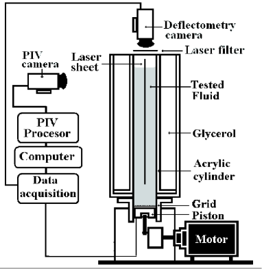
Figure 1: Schematic view of the experimental device, including the setups for PIV and deflectometry measurements.

Thus,

$$\frac{dp(t)}{dz}=\rho z_{0}\omega^{2}\sin(\omega t).$$ (2)

The velocity profile in the radial direction of the tube, at the driving frequency $\omega$, is then given by the real part of the following expression:

$$v(r,t)=-i\left(1-\frac{J_{0}(\beta r)}{J_{0}(\beta a)}\right)z_{0}\omega e^{i\omega t}.$$ (3)

For a Newtonian fluid ($t_{m}=0$) there is only one node of the velocity profile, at $r=a$, which accounts for the non–slip condition at the wall. Remarkably, if $t_{m}\neq 0$ (Maxwellian fluid) the velocity profile may present several nodes. These nodes define quiescent points of the flow. For given material and geometrical parameters, the location of the nodes depends on the driving frequency, as shown in Fig. 2.

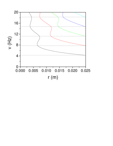
Figure 2: Diagram showing the location of the quiescent flow points along the radial coordinate of the cylinder, $r$, as a function of driving frequency, $\nu$, for a Maxwell fluid. The dashed horizontal lines separate the frequency axis in intervals of constant number of quiescent flow points. The parameters $\rho$, $t_{m}$, and $\eta$ used to compute the diagram are the ones listed in the text for the 60/100 CPyCl/NaSal solution, together with the cylinder radius $a=25$ mm.

As mentioned in the Introduction, the elastic properties of the fluid dominate the dynamic response of the system at the resonant frequencies. In Eq. (3) this is manifest in that, at the resonant frequencies, the oscillation in the centre of the tube (maximum velocity) is in phase with the driving.

III Experimental device

The experimental device is shown in Fig. 1. The cylindrical container (inner radius $a=25$ mm, length 500 mm) is made of transparent acrylic. In order to avoid optical aberrations this cylinder is placed inside a second recipient of square section, made also of transparent acrylic, which is filled with glycerol to match the refractive index of the acrylic walls. A Teflon piston driven by a motor of variable frequency produces harmonic oscillations of the pressure gradient in the liquid column. Although the motor controller can operate in the frequency range from $1.5$ to 200 Hz, our experiments have been performed in the reduced frequency range from $1.5$ to 15 Hz. The piston oscillation amplitude is set to $0.80\pm 0.05$ mm to keep the Reynolds number low, within the accessible frequency range, for the two fluids studied. Additional details of this part of the setup are described in Ref. Castrejon03 .

The viscoelastic fluid used in these experiments is an aqueous solution of cetylpyridinium chloride and sodium salicylate (CPyCl/NaSal). This surfactant solution is known to exhibit the rheological behaviour of a linear Maxwell fluid in a range of concentrations Hoffman91 ; Berret93 . In most experiments we have used a 60/100 concentration, for which the dynamic viscosity $\eta=60$ Pa$\cdot$s, the density $\rho=1050$ kg/m³, and the relaxation time $t_{m}=1.9$ s MendezSanchez03 . In DLA measurements we have also used a 40/40 concentration, for which $\eta=30$ Pa$\cdot$s, $\rho=1005$ kg/m³, and relaxation time around $t_{m}=1.25$ s. Our rheological characterisation of this last fluid, however, suggests that it cannot be fully described by a single relaxation time. As Newtonian fluid we have used commercial glycerol, with nominal dynamic viscosity $\eta=1$ Pa$\cdot$s and density $\rho=1250$ kg/m³. These values have been determined at the working temperature of $(25\pm 0.5)^{\circ}$C.

All sets of measurements performed on the same fluid have been carried out in order of increasing frequency. The cylinder has been emptied and refilled with fresh fluid every time that a series of measurements at three different driving frequencies was complete, i.e. approximately every day. Measurements in the bulk have been carried out at two different heights, corresponding to distances of 6 and 10 cm from the upper free interface.

The LDA technique used in the measurements presented in the next Section has already been described in detail in Ref. Castrejon03 . We present now a brief description of the other two techniques (PIV and deflectometry).

III.1 Particle Image Velocimetry

The PIV technique provides instant measures of the velocity maps in a plane of the flow Adrian91 . To this purpose, the fluid is seeded with small particles. The velocity maps are obtained by a measure of the statistical correlation of the displacement of the seeding particles in the fluid in a known time interval, in this case the time between two consecutive laser pulses.

Our PIV system contains a two pulsed Nd-YAG lasers unit, that includes an optical array to produce a laser light sheet in a vertical plane of the acrylic cylinder (Fig. 1). A high resolution camera (Kodak E1.0), perpendicular to the laser light sheet, is used to record the digital images. The camera records two consecutive frames, one corresponding to each laser light pulse. The acquisition rate is limited by the camera to three pairs of images every two seconds (1.5 Hz). A Dantec FlowMap 1100 processor takes care of the synchronization between the laser pulses and the camera trigger. Post–processing of the data, to determine velocity maps, is carried out by the Dantec FlowMap v5.1 software. Dantec 20–$\mu$m polyamid spheres were used as seeding particles in the present experiments. These particles are small enough to follow the flow with minimal drag, but sufficiently large to scatter enough light to obtain good particle images.

III.2 Optical Deflectometry

Deflectometry is a technique used to study relatively small deformations in transparent fluid surfaces Fermigier92 . In our case the liquid column serves as a variable–thickness lens. A thin transparent plastic sheet with a regular array (grid spacing $d$) of black dots (0.5 mm diameter) is placed on top of the Teflon piston, at the bottom of the acrylic cylinder (Fig. 1). The grid is imaged through the liquid column using a CCD camera interfaced to a computer. Light passing through the liquid column is refracted at the liquid–air interface, distorting the image of the grid as the interface deforms. Figure 3 presents an example of the recorded images.

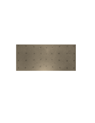
Figure 3: A typical picture recorded in Optical Deflectometry measurements. The image of a regular array of black dots (grid spacing $d=5.0$ mm) is distorted by the interface deformation.

The displacement of an imaged grid point, $\delta$, is related to the local slope of the interface, $\phi$, in the following way (Fig. 4). According to Snells’ refraction law, $n_{1}\theta=n_{2}\phi$. On the other hand, for a column height $h$ the figure shows that $\tan(\phi-\theta)=\delta/h$. Therefore, the relation between $\phi$ and $\delta$ reads:

$$\phi=\frac{1}{1-n_{2}/n_{1}}\arctan\left(\frac{\delta}{h}\right).$$ (4)

In our setup the height of the liquid column ($H=240$ mm) is much larger than the local height variations produced by the deformation of the interface (of the order of mm), and we can safely take $h\simeq H$ in Eq. (4).

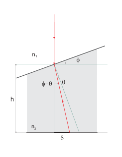
Figure 4: Sketch of the path followed by a light ray in the system.

OD is usually used in thin films. The deflection of the points of the grid increases with the depth of the layer, making this technique useless for the measurement of highly deformed interfaces of thick layers. However, the small amplitude of the perturbation in our experiments generates relatively smooth profiles, and the condition of small deformations is satisfied in a wide range of frequencies.

Although the deformations are small in this frequency range, the whole deformation profile depends strongly on the frequency of driving. This can be seen on the theoretical deformation profiles of the viscoelastic fluid at 2 and $6.5$ Hz, displayed in Fig. 5. The two profiles are very different. While the deformation profile at 2 Hz is monotonic and very smooth, the profile at $6.5$ Hz shows a more complex behaviour: instead of a single central node, it presents two nodes which, in the velocity profile, correspond to a maximum at the tube centre and a minimum near the tube wall. The maximum deformation between these two nodes corresponds to an inflection point of the velocity profile, very close to the quiescent flow point.

Figure 5: Theoretical deformation profiles of the Maxwell fluid driven at 2 Hz (dashed line) and at $6.5$ Hz (solid line).

In our setup the height of the liquid column is a function of the radial coordinate $r$, and periodic in time. This height, $h(r,t)$, is simply related to the local slope by $\phi(r,t)=\partial h(r,t)/\partial r$. Hence:

$$h(r,t)=h(r_{0},t)+\int_{r_{0}}^{r}\phi(r,t)\,dr.$$ (5)

It is useful to choose for $r_{0}$ a position where the interface is motionless, because the reference height $h(r_{0},t)$ is then a constant that can be taken equal to 0. We have chosen $r_{0}$ as the radial coordinate of the quiescent flow point (in the bulk) closest to the cylinder axis. Implicitly, we are assuming that the stagnation points predicted by Eq. (3) for the bulk do not change their position as the interface is approached. This assumption is confirmed by our PIV and OD results (see Sec. IV).

Finally, the velocity profile of the interface can be obtained from the time derivative of the local height, $v(r,t)=\partial h(r,t)/\partial t$.

In our experiments the grid spacings used are $d=5.0$ and $5.5$ mm, and the refractive indices are $n=1.33407(01)$ for the CPyCl/NaSal solution (measured by Abbé refractometry), and $n=1.473$ for glycerol (nominal).

IV Results and discussion

IV.1 rms velocity at the cylinder axis

The amplitude of the velocity field given by Eq. (1) presents resonance peaks at several resonance frequencies. As mentioned in the Introduction, this phenomenon was demonstrated experimentally and compared to the purely dissipative behaviour of a Newtonian fluid in Ref. Castrejon03 . These results showed that the linear theory gives a good prediction of the resonance frequencies but overestimates the amplitude of the resonance peaks.

We have repeated this same kind of measurements in the present work, to check the dependence of the resonance frequencies on the rheological properties of the Maxwell fluid. To this purpose the driving frequency $\omega$ has been rescaled by a characteristic time $\tau$ defined as

$$\tau=10^{2/5}t_{m}\sqrt{\alpha},$$ (6)

where $\alpha$ is the inverse of our Deborah number $De=t_{m}\eta/a^{2}\rho$. As it was shown in Ref. delRio98 , the location of the resonance peaks becomes universal (independent of fluid parameters and system dimensions) if $\omega$ is made dimensionless in the form $\omega\tau$.

Then, we rewrite Eq. (1) in the form

$$V(r,\omega)=\xi(r,\omega)\frac{dP}{dz},$$ (7)

and plot the dimensionless response function $\xi(r,\omega)/\xi(r,0)$ as a function of the dimensionless driving fequency $\omega\tau$. The results at the centre of the tube ($r=0$), for the two different concentrations of the CPyCl/NaSal solution used, are shown in Fig. 6. Comparison with the linear theory is given by the vertical dashed lines, which give the resonance frequencies corresponding to maxima of $\xi(r=0,\omega)$. The Figure shows that the rescaling of the frequency axis suggested by the linear theory leads to a satisfactory reproducibility of the resonance frequencies independently of viscoelastic fluid parameters.

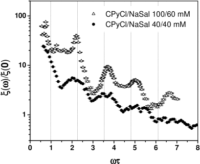
Figure 6: Dimensionless response function at the centre of the cylinder, as a function of dimensionless driving frequency, for two concentrations of the CPyCl/NaSal solution. The vertical dashed lines give the location of the resonance frequencies predicted by a linear theory.

The magnitude of the response function at the resonance peaks for the surfactant solution of concentration 60/100 is considerably lower in the present measurements than in the previous ones of Ref. Castrejon03 . The reason is that the present measurements have been carried out at 6 cm of the free air–liquid interface, while the previous ones had been taken at 10 cm. The different measured velocities provide a first evidence of the damping influence of the free interface on the flow.

The results presented in the next two sections provide measurements of the whole velocity profile, instead of measurements at a single point in the flow Castrejon03 . The velocity profiles are obtained at two different heights, in the bulk of the fluid, and at the fluid-air interface.

IV.2 Velocity profiles in the bulk

The following set of figures presents the velocity profiles in the bulk of the fluid column, determined by PIV measurements, together with the theoretical profiles given by Eq. (3) at coincident time–phases, for comparison. The profiles have been determined at the driving frequencies of $2$ Hz (Figs. 7 and 8), $6.5$ Hz (Figs. 9 and 10), and $10$ Hz (Figs. 11 and 12). These values coincide with the first three resonance frequencies of our system for the 60/100 viscoelastic solution, as given by Eq. (3). The time–phases have been selected by the criterion that the velocity at the tube axis is a maximum.

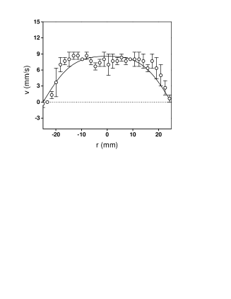
Figure 7: Glycerol: PIV results at 2 Hz (dots), measured at 6 cm from the upper free interface, and the corresponding theoretical prediction (solid line) at $t=0.125$ s.

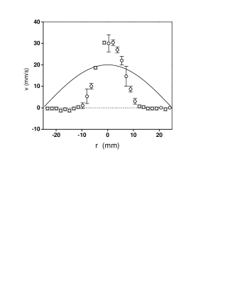
Figure 8: 60/100 CPyCl/NaSal solution: PIV results at 2 Hz (dots), measured at 6 cm from the upper free interface, and the corresponding theoretical prediction (solid line) at $t=0.375$ s.

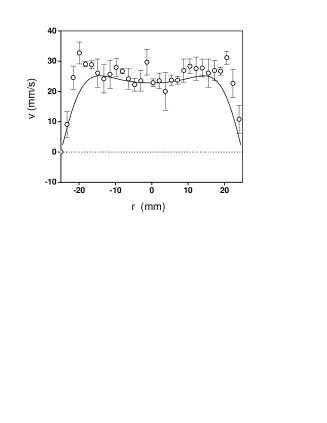
Figure 9: Glycerol: PIV results at 6.5 Hz (dots), measured at 6 cm from the upper free interface, and the corresponding theoretical prediction (solid line) at $t=0.115$ s.

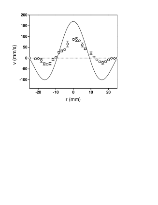
Figure 10: 60/100 CPyCl/NaSal solution: PIV results at 6.5 Hz (dots), measured at 6 cm from the upper free interface, and the corresponding theoretical prediction (solid line) at $t=0.038$ s.

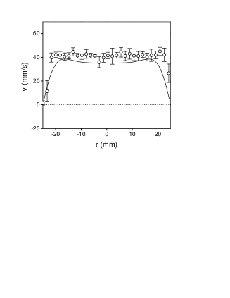
Figure 11: Glycerol: PIV results at 10 Hz (dots), measured at 6 cm from the upper free interface, and the corresponding theoretical prediction (solid line) at $t=0.075$ s.

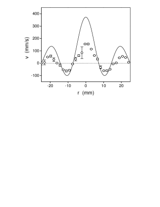
Figure 12: 60/100 CPyCl/NaSal solution: PIV results at 10 Hz (dots), measured at 6 cm from the upper free interface, and the corresponding theoretical prediction (solid line) at $t=0.025$ s.

The first observation to make is that the instantaneous velocity profiles of the Maxwell fluid, driven at 2 Hz, present a single defined sign of velocity (single direction of motion) along the whole radius of the tube. As the driving frequency is increased to 6.5 and 10 Hz, however, the instantaneous profiles display a progressively more complex structure, revealing the presence of annular regions within the tube with alternating upward/downward motion. Notice that this complexity is inherent to the viscoelastic properties of the Maxwell fluid. For the Newtonian fluid (glycerol) the instantaneous flow in the tube goes all in the same direction for the three driving frequencies tested.

For the viscoelastic fluid the frontiers between consecutive annular regions with alternating signs of the velocity do not move. They correspond to the stagnation regions of the flow which were already discussed in the context of the linear theory. The PIV results show that the number of quiescent flow points along the radial direction of the tube increases with the driving frequency, in agreement with the theoretical prediction (Fig. 2).

Some of the measured profiles of the viscoelastic fluid show regions near the walls with vanishingly small velocities and near zero velocity gradients, most noticeably the one at 2 Hz shown in Fig. 8. These profiles are reminiscent of velocity profiles obtained for systems that display shear–banding. Indeed, the CPyCl/NaSal solution is commonly known to show shear-banding Lourdes2 , but we have enough evidence to discard this effect in our experiments. We did not observe an increase in turbidity in the region of the fluid close to the walls, nor changes in the local intensity of the scattered light that could be attributed to inhomogeneities. Furthermore, we monitored possible changes on the polarization state of the scattered light, an indication of banding shear–banding . No changes in the optical properties were observed for the amplitude and frequency range used here. In addition, Fig. 13 demonstrates that the velocity near the walls takes values distinctly different from zero at different phases within an oscillation period.

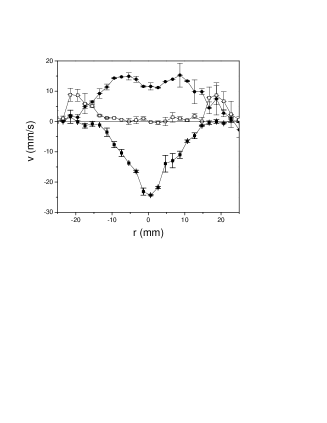
Figure 13: 60/100 CPyCl/NaSal solution: PIV results at 2 Hz, measured at 6 cm from the upper free interface and at different time phases within a driving period.

Performing PIV measurements at two different heights of the liquid column allows studying the influence of the upper free interface on the velocity profiles. Thus, it is interesting to compare the results presented above, which have been performed at 6 cm from the upper interface, to the results shown in Figs. 14 and 15, which have been performed at 10 cm from the upper interface. The first conclusion to draw from corresponding measurements at different heights is that the location of the quiescent flow points is not affected by the presence of the upper free interface. The second conclusion is that the magnitude of the velocity profile is smaller when the measurement is carried out closer to the free interface. The damping effect of the free interface, disregarded in the theory, originates from the air–liquid surface tension. This observation applies equally to the two fluids investigated (Newtonian and Maxwellian).

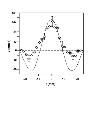
Figure 14: 60/100 CPyCl/NaSal solution: PIV results at 6.5 Hz (dots), obtained at 10 cm from the upper free interface, and the corresponding theoretical prediction (solid line) at $t=0.057$ s.

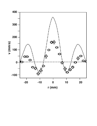
Figure 15: 60/100 CPyCl/NaSal solution: PIV results at 10 Hz (dots), obtained at 10 cm from the upper free interface, and the corresponding theoretical prediction (solid line) at $t=0.022$ s.

The experimental velocity profiles are in reasonable agreement with the theoretical ones. The number of quiescent flow points is the same, and their location very similar. As a general trend, however, the theory overestimates the measured velocity.

A first explanation would be that the theory disregards nonlinearities, and these tend to limit the largest velocity values. Nonlinearities could arise from either the hydrodynamic equations or the constitutive relation of the fluid. In our case, however, since the small amplitude of the piston oscillations ensures that Re$<$ 10^-4, the linearized momentum equation is a very good approximation. On the other hand, taking into account the cylindrical symmetry of the problem and assuming that the velocity depends only on the radial coordinate (as our results confirm to a very good approximation), it turns out that the first nonlinear correction to the constitutive equation of the fluid cancels out exactly.

The disagreement between theory and experiment is probably due to shear–thinning of the viscoelastic fluid. As shown in Ref. MendezSanchez03 , our fluid is properly described by a Maxwell model up to shear rates $\gamma\simeq 0.6$ s^-1, and experiences shear–thinning beyond that value. A close inspection of Figs. 8, 10, and 12 reveals that the shear rate actually experienced by the fluid in some phase intervals of the oscillation is larger Castrejon03 . In these conditions the viscosity of the fluid decreases with shear. The theory predicts that the dynamic response of the system at the resonant frequencies becomes smaller as the viscosity is reduced delRio98 , and thus would support the view that the measured velocity profiles are systematically smaller than the theoretical ones for the viscoelastic fluid (and not for the newtonian fluid) because of shear–thinning.

IV.3 Deflection of the air–liquid interface

The results obtained by Optical Deflectometry are presented on top of Figs. 16 and 17 (2 Hz), and Figs. 18 and 19 ($6.5$ Hz). There are no results at 10 Hz because, at this driving frequency, the deformations of the free interface of the Maxwellian fluid are so large that the technique is not applicable. Each figure displays measurements at two different time–phases.

The experimental deformation profiles of the interface at $2$ and $6.5$ Hz for the viscoelastic fluid can be compared to the theoretical ones (computed for the bulk) displayed in Fig. 5. We observe that their shapes are fully coincident for each of the two driving frequencies. This shows that the quiescent flow points of the velocity profiles do not change their position along the vertical direction, and thus their location in the bulk can be used as reference to compute the velocity profiles at the interface from the deformation profiles.

The velocity profiles are presented on the bottom of Figs. 16 and 17 (2 Hz), and Figs. 18 and 19 ($6.5$ Hz). The magnitude of the interfacial velocities is in all cases much lower than the one measured in the bulk of the fluid. This is mostly due to the stabilizing role of surface tension, as discussed above.

It is interesting to note that the velocity profiles of the interface depend also on the direction of motion of the driving piston. The magnitude of the velocity is systematically lower for positive displacements of the piston (liquid displacing air) than for negative ones (air displacing liquid). We attribute this asymmetry to the fact that the large viscosity contrast across the interface stabilizes the displacement of a nearly inviscid fluid (air) by a viscous liquid, and destabilizes the opposite displacement.

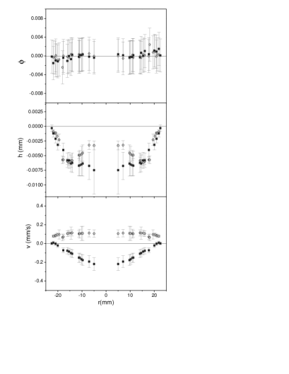
Figure 16: Glycerol: deflectometry results at 2 Hz, measured at two different time–phases within an oscillation.

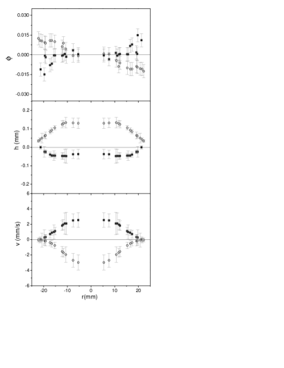
Figure 17: 60/100 CPyCl/NaSal solution: deflectometry results at 2 Hz, measured at two different time–phases within an oscillation.

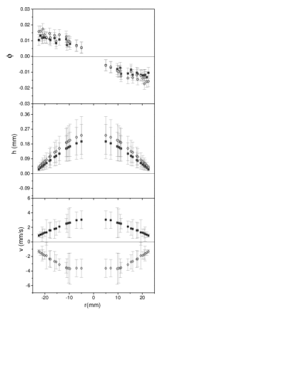
Figure 18: Glycerol: deflectometry results at 6.5 Hz, measured at two different time–phases within an oscillation.

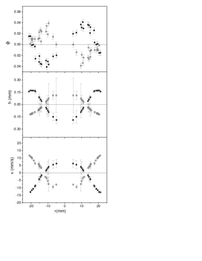
Figure 19: 60/100 CPyCl/NaSal solution: deflectometry results at 6.5 Hz, measured at two different time–phases within an oscillation.

V Conclusions

We have used three different optical techniques to characterize the oscillating flow of a viscoelastic fluid (a solution of CPyCl/NaSal in water) contained in a vertical cylinder and subjected to an oscillating pressure gradient. A Newtonian fluid (glycerol) has also been studied for the sake of comparison.

LDA measurements of the fluid velocity at the symmetry axis of the cylinder as a function of driving frequency, for two different compositions of the surfactant solution, have enabled us to show that the frequencies of the resonance peaks can be predicted accurately in terms of the fluid rheological properties by a simple linear theory. This theory neglects inertial effects, and makes use of a linear Maxwell model as constitutive relation for the viscoelastic fluid.

Systematic PIV measurements of the radial velocity field in the bulk of the fluid have been performed at three different driving frequencies, close to the first three resonance frequencies of the viscoelastic system. While the velocity profile of the Newtonian fluid along the radial direction does not change sign, this is not the case for the Maxwellian fluid. The profiles measured at $6.5$ and 10 Hz present regions with alternating signs of the velocity, separated by quiescent flow points. The number of quiescent flow points increases with the driving frequency, revealing the increasing complexity of the flow. Measurements within the fluid column at two different heights show that these quiescent flow points do not shift as one moves along the vertical direction, and that their radial location is accurately reproduced by the linear theory.

The presence of a free interface at the top of the liquid column has a damping effect on the velocity amplitude. This observation is visible, both with LDA and PIV, when the results of measurements carried out at two different heights within the liquid column are compared.

Optical Deflectometry measurements of the free interface confirm that the velocity field is severely damped by the surface tension of the air–liquid interface, compared to the velocity field within the bulk. Interestingly, the deflectometry results show also that the oscillations of the velocity field at the interface are asymmetric, the profiles corresponding to positive displacements of the piston having a slightly but systematically smaller amplitude than those corresponding to negative displacements. We attribute this asymmetry to the fact that the upward motion of the interface (liquid displacing air) is stabilized by the viscous pressure gradient in the liquid. Recently it has been suggested that the viscous fingering interfacial instability of a viscoelastic fluid in a Hele–Shaw cell will be enhanced by making the flow oscillate at the resonant frequencies Corvera04 . Our deflectometry results show that the stabilizing role of the surface tension will reduce this effect to some extent.

These results, as part of the study of resonance frequencies in viscoelastics, are potentially relevant in biorheology to interpret the frequencies at which biofluids are optimally pumped in living organisms Lambert04 .

VI Acknowledgements

We acknowledge A. Morozov (Universiteit Leiden) for illuminating discussions, and J. Soriano (Universität Bayreuth) and G. Hernández (UNAM) for their technical assistance. This research has received financial support through projects BQU2003-05042-C02-02 and BFM2003-07749-C05-04 (MEC, Spain), SGR-2000-00433 (DURSI, Generalitat de Catalunya), and CONACyT 38538 (Mexico). JO acknowledges additional support from the DURSI. JRCP acknowledges the support by CONACyT, SEP, and the ORS Award Scheme. AACP acknowledges the support given by the Dorothy Hodgkin Award.

References

- (1) For an overview, see W.M. Gelbart and A. Ben–Shaul, J. Phys. Chem. 100, 13169 (1996).
- (2) R.G. Larson, The Structure and Rheology of Complex Fluids (Oxford University, Oxford, 1999).
- (3) M. López de Haro, J.A. del Río, and S. Whitaker, in Lectures on Thermodynamics and Statistical Mechanics, edited by M. Costas, R.F. Rodríguez, and A.L. Benavides (World Scientific, Singapore, 1994), pp. 54–70.
- (4) M. López de Haro, J.A. del Río, and S. Whitaker, Transp. Porous Media 25, 167 (1996).
- (5) J.A. del Río, M. López de Haro, and S. Whitaker, Phys. Rev. E 58, 6323 (1998); 64, 039901 (E) (2001).
- (6) D. Tsiklauri and I. Beresnev, Phys. Rev. E 63, 046304 (2001).
- (7) J.R. Castrejón–Pita, J.A. del Río, A.A. Castrejón–Pita, and G. Huelsz, Phys. Rev. E 68, 046301 (2003).
- (8) J.A. del Río and J.R. Castrejón–Pita, Rev. Mex. Fís. 49, 75 (2003).
- (9) R.H. Hoffman, Mol. Phys. 75, 5 (1991).
- (10) J.F. Berret, J. Apell, and G. Porte, Langmuir 9, 2851 (1993).
- (11) A.F. Méndez–Sánchez, M.R. López–González, V.H. Rolón–Garrido, and J. Pérez–González, and L. de Vargas, Rheol. Acta 42, 56 (2003).
- (12) R.J. Adrian, Annu. Rev. Fluid Mech. 23, 261 (1991).
- (13) M. Fermigier, L. Limat, J.E. Wesfreid, P. Boudinet, and C. Quilliet, J. Fluid Mech. 236, 349 (1992).
- (14) A.F. Méndez-Sánchez, J. Pérez–González, L. de Vargas, J.R. Castrejón–Pita, A.A. Castrejón–Pita, and G. Huelsz, J. of Rheology 47, 1455 (2003).
- (15) S. Lerouge and J.P. Decruppe, Langmuir 16, 6464 (2000).
- (16) E. Corvera Poiré and J.A. del Río, J. Phys.: Condens. Matter 16, S2055 (2004).
- (17) A.A. Lambert, G. Ibáñez, S. Cuevas, and J.A. del Río, Phys. Rev. E 70, 056302 (2004).