A variance-minimization scheme for optimizing Jastrow factors

Abstract

We describe a new scheme for optimizing many-electron trial wave functions by minimizing the unreweighted variance of the energy using stochastic integration and correlated-sampling techniques. The scheme is restricted to parameters that are linear in the exponent of a Jastrow correlation factor, which are the most important parameters in the wave functions we use. The scheme is highly efficient and allows us to investigate the parameter space more closely than has been possible before. We search for multiple minima of the variance in the parameter space and compare the wave functions obtained using reweighted and unreweighted variance minimization.

I Introduction

Accurate many-body wave functions are essential to the variational and diffusion quantum Monte Carlo (VMC and DMC) methods, as the wave function controls both the statistical efficiency and the accuracy of these techniques.foulkes_2001 Optimizing many-body wave functions is perhaps the most important technical issue facing practitioners of these quantum Monte Carlo (QMC) techniques today, and it consumes large quantities of human and computing resources.

Wave-function optimization schemes have usually involved minimizing either the variational energy or its variance. Although it is generally believed that wave functions corresponding to the minimum energy have more desirable properties, variance minimization has been very widely used because it has proved easier to design robust minimization techniques for this purpose.umrigar_1988a ; kent_1999 The scheme introduced in this article involves minimizing the unreweighted variance. We describe a new method for evaluating this quantity, which greatly accelerates the optimization of parameters that occur in a linear fashion in the exponent of a Jastrow factor. These are, in general, the most important parameters in QMC trial wave functions. The optimization step does not involve a sum over electron configurations, which means that we can use very large numbers of configurations. The unreweighted variance is in fact a quartic function of the linear parameters in the Jastrow factor, and the minima of multidimensional quartic functions can be located very rapidly. The efficiency of our scheme has enabled us to explore the minimization procedure and the parameter space in detail, and to investigate the possible existence of multiple minima.

The distinction between the reweighted or true variance and the unreweighted variance is explained in Sec. II. In Sec. III we describe our accelerated scheme for calculating the unreweighted variance. In Sec. IV we use our new method to study the unreweighted variance in parameter space. The minima of the reweighted and unreweighted variance need not coincide, and in Sec. V we investigate which minimum corresponds to the lower energy. We discuss the sampling of configuration space and the flexibility of the trial wave function in Secs. VI and VII. In Secs. IX and X we compare the efficiency of the “standard” and accelerated variance-minimization methods, both in theory and practice. Finally, we draw our conclusions in Sec. XI.

Hartree atomic units (a.u.) are used throughout, in which the Dirac constant, the magnitude of the electronic charge, the electronic mass, and $4\pi$ times the permittivity of free space are unity: $\hbar=|e|=m_{e}=4\pi\epsilon_{0}=1$. All of our QMC calculations were carried out using the casino package.casino

II The energy and its variance

Consider a real trial wave function $\Psi({\bf R})$, where ${\bf R}$ is a point in the electron configuration space. In VMC the energy is written as

$$E=\frac{\int\Psi({\bf R})^{2}E_{L}({\bf R})\,d{\bf R}}{\int\Psi({\bf R})^{2}\,d{\bf R}},$$ (1)

where the local energy, $E_{L}$, is

$$E_{L}({\bf R})=\Psi({\bf R})^{-1}\hat{H}({\bf R})\Psi({\bf R}),$$ (2)

and $\hat{H}$ is the Hamiltonian. The variance of the energy is

$$\sigma^{2}=\frac{\int\Psi({\bf R})^{2}(E_{L}({\bf R})-E)^{2}\,d{\bf R}}{\int\Psi({\bf R})^{2}\,d{\bf R}}.$$ (3)

We write the trial wave function as $\Psi^{\{\alpha\}}({\bf R})$, to denote that it depends on a set of free parameters, $\{\alpha\}$. Throughout this article, we confine our attention to the optimization of parameters in the Jastrow factor. The nodal surface of the trial wave function is independent of such parameters. Consider a set of $N_{C}$ configurations $\{{\bf R}\}$ distributed according to $\left(\Psi^{\{\alpha_{0}\}}({\bf R})\right)^{2}$ for some fixed parameter set $\{\alpha_{0}\}$. The variance $\sigma^{2}$ is then estimated for any given parameter set $\{\alpha\}$ using a correlated-sampling procedure, which gives rise to the reweighted variance,

$$\sigma_{w}^{2}=\frac{T_{\{\alpha_{0}\}}^{\{\alpha\}}}{\left(T_{\{\alpha_{0}\}}^{\{\alpha\}}\right)^{2}-\sum_{\bf R}\left(W_{\{\alpha_{0}\}}^{\{\alpha\}}({\bf R})\right)^{2}}\sum_{\bf R}\left(E_{L}^{\{\alpha\}}({\bf R})-\bar{E_{w}}\right)^{2}W_{\{\alpha_{0}\}}^{\{\alpha\}}({\bf R}),$$ (4)

where the reweighted energy is

$$\bar{E}_{w}=\frac{1}{T_{\{\alpha_{0}\}}^{\{\alpha\}}}\sum_{\bf R}E_{L}^{\{\alpha\}}({\bf R})W_{\{\alpha_{0}\}}^{\{\alpha\}}({\bf R}),$$ (5)

which is an estimate of $E$, and the total weight is

$$T_{\{\alpha_{0}\}}^{\{\alpha\}}=\sum_{\bf R}W_{\{\alpha_{0}\}}^{\{\alpha\}}({\bf R}),$$ (6)

and the weights $W$ are

$$W_{\{\alpha_{0}\}}^{\{\alpha\}}({\bf R})=\left(\frac{\Psi^{\{\alpha\}}({\bf R})}{\Psi^{\{\alpha_{0}\}}({\bf R})}\right)^{2}.$$ (7)

The unreweighted variance as a function of parameter set $\{\alpha\}$ is defined to be

$$\sigma_{u}^{2}=\frac{1}{N_{C}-1}\sum_{\bf R}\left(E_{L}^{\{\alpha\}}({\bf R})-\bar{E_{u}}\right)^{2},$$ (8)

where the unreweighted energy is

$$\bar{E_{u}}=\frac{1}{N_{C}}\sum_{\bf R}E_{L}^{\{\alpha\}}({\bf R}).$$ (9)

The reweighted and unreweighted variances are identical when the same set of configurations is used and ${\{\alpha\}}={\{\alpha_{0}\}}$. However, for any given ${\{\alpha_{0}\}}$ they are different functions of ${\{\alpha\}}$, and there is no reason to expect that their minima coincide with each other, or that either minimum should coincide with that of the (reweighted) energy.

Both $\sigma_{w}^{2}$ and $\sigma_{u}^{2}$ are non-negative, but are zero when $\Psi^{\{\alpha\}}$ is an eigenstate of $\hat{H}$. The reweighted and unreweighted variances are therefore reasonable cost functions for wave-function optimizations. The reweighted energy is also a reasonable cost function. However, the problem with the reweighted energy and variance is that the weights $W$ may vary rapidly as the parameters change, especially for large systems, which leads to instabilities in optimization procedures.kent_1999 It can be shown that the wave function used to generate the configuration set corresponds to a stationary point of $\bar{E_{u}}$ (for perfect sampling). In what follows we will mainly be interested in optimizing linear parameters in the Jastrow factor, and in this case we have proved that the wave function used to generate the configuration set corresponds to the global maximum of the unreweighted energyfootnote_unreweighted_energy . The unreweighted energy is clearly not a suitable cost function. From these considerations we conclude that the cost function with the most suitable mathematical properties for the stable optimization of wave functions within the correlated-sampling approach is the unreweighted variance.

The usual variance-minimization procedure is to generate a set of electron configurations $\{{\bf R}\}$ distributed according to $\left(\Psi^{\{\alpha_{0}\}}({\bf R})\right)^{2}$ using VMC, and then to minimize the reweighted or unreweighted energy variance over this set. Since the variance landscape depends on the distribution of configurations, several cycles of configuration generation and optimization are normally carried out, with the optimized wave function from the previous cycle being used in each VMC configuration-generation phase. We usually iterate several times and choose the wave function that gives the lowest variational energy. In the limit of perfect sampling, the reweighted variance is equal to the actual variance, and is therefore independent of the configuration distribution, so that the optimized parameters would not change over successive cycles of reweighted variance minimization. This is not the case for unreweighted variance minimization; nevertheless, by carrying out a number of cycles, a “self-consistent” parameter set may be obtained.

III Accelerated evaluation of the unreweighted variance

III.1 The Slater-Jastrow wave function

Let $\Psi$ be a Slater-Jastrow wave function for a many-body system:

$$\Psi({\bf R})=\exp[J({\bf R})]S({\bf R}),$$ (10)

where $\exp[J]$ is the Jastrow factor, which contains free parameters to be determined by an optimization method, and $S$ is the Slater wave function, which may be an expansion in several determinants of single-particle orbitals.

Suppose that $J$ contains linear parameters $\alpha_{1},\ldots,\alpha_{P}$, that is,

$$J({\bf R})=\sum_{i=1}^{P}f_{i}({\bf R})\alpha_{i}+J_{0}({\bf R}),$$ (11)

where $f_{1},\ldots,f_{P}$ and $J_{0}$ are known functions of ${\bf R}$, which depend upon the particular form of Jastrow factor used and do not contain any free parameters. We use the form of Jastrow factor described in detail in Ref. ndd_jastrow , which contains linear parameters. However, some of the terms have a finite extent in space and the associated cutoff lengths must appear nonlinearly in the Jastrow factor. These cutoff lengths can be set on physical grounds or optimized using small numbers of parameters and configurations and the standard variance-minimization procedure, but their values cannot be obtained using the accelerated scheme described here.

III.2 Derivation of the quartic polynomial

The local energy for the Slater-Jastrow wave function of Eq. (10) is

$$E_{L}({\bf R})=-\frac{1}{2}\sum_{i=1}^{P}\sum_{j=1}^{P}g_{ij}^{(2)}({\bf R})\alpha_{i}\alpha_{j}-\frac{1}{2}\sum_{i=1}^{P}g_{i}^{(1)}({\bf R})\alpha_{i}-\frac{1}{2}g^{(0)}({\bf R})+V({\bf R}),$$ (12)

where $V$ is the potential energy and

$$g_{ij}^{(2)}({\bf R}) = \nabla f_{i}\cdot\nabla f_{j}$$ (13)

$$g_{i}^{(1)}({\bf R}) = 2\nabla f_{i}\cdot\nabla J_{0}+\nabla^{2}f_{i}+2\frac{\nabla S}{S}\cdot\nabla f_{i}$$ (14)

$$g^{(0)}({\bf R}) = |\nabla J_{0}|^{2}+\nabla^{2}J_{0}+2\frac{\nabla S}{S}\cdot\nabla J_{0}+\frac{\nabla^{2}S}{S},$$ (15)

and we note that $g_{ij}^{(2)}=g_{ji}^{(2)}$. The square of the local energy is given by

$$E_{L}^{2}({\bf R}) = \sum_{i=1}^{P}\sum_{j=1}^{P}\sum_{k=1}^{P}\sum_{l=1}^{P}G_{ijkl}^{(4)}({\bf R})\alpha_{i}\alpha_{j}\alpha_{k}\alpha_{l}+\sum_{i=1}^{P}\sum_{j=1}^{P}\sum_{k=1}^{P}G_{ijk}^{(3)}({\bf R})\alpha_{i}\alpha_{j}\alpha_{k}$$ (16)

$${}+\sum_{i=1}^{P}\sum_{j=1}^{P}G_{ij}^{(2)}({\bf R})\alpha_{i}\alpha_{j}+\sum_{i=1}^{P}G_{i}^{(1)}({\bf R})\alpha_{i}+G^{(0)}({\bf R}),$$

where

$$G_{ijkl}^{(4)}({\bf R}) = \frac{g_{ij}^{(2)}({\bf R})g_{kl}^{(2)}({\bf R})}{4}$$ (17)

$$G_{ijk}^{(3)}({\bf R}) = \frac{g_{ij}^{(2)}({\bf R})g_{k}^{(1)}({\bf R})}{2}$$ (18)

$$G_{ij}^{(2)}({\bf R}) = \frac{g_{i}^{(1)}({\bf R})g_{j}^{(1)}({\bf R})}{4}-g_{ij}^{(2)}({\bf R})\left(V({\bf R})-\frac{g^{(0)}({\bf R})}{2}\right)$$ (19)

$$G_{i}^{(1)}({\bf R}) = -g_{i}^{(1)}({\bf R})\left(V({\bf R})-\frac{g^{(0)}({\bf R})}{2}\right)$$ (20)

$$G^{(0)}({\bf R}) = \left(V({\bf R})-\frac{g^{(0)}({\bf R})}{2}\right)^{2}.$$ (21)

(Note that $G_{ijkl}^{(4)}=G_{jikl}^{(4)}=G_{ijlk}^{(4)}=G_{klij}^{(4)}$, $G_{ijk}^{(3)}=G_{jik}^{(3)}$, and $G_{ij}^{(2)}=G_{ji}^{(2)}$.)

Suppose the VMC method is used to generate a set of $N_{C}$ points in configuration space, $\{{\bf R}\}$, which are distributed according to the square of an approximate trial wave function. For any quantity $A({\bf R})$, let

$$\bar{A}=\frac{1}{N_{C}}\sum_{\bf R}A({\bf R})$$ (22)

be the average of $A({\bf R})$ over the set of $N_{C}$ configurations. The unreweighted variance may be written as

$$\sigma_{u}^{2} = \frac{N_{C}}{N_{C}-1}\left(\bar{E_{L}^{2}}-\bar{E_{L}}^{2}\right)$$ (23)

$$\equiv \frac{N_{C}}{N_{C}-1}\left(\sum_{i=1}^{P}\sum_{j=1}^{P}\sum_{k=1}^{P}\sum_{l=1}^{P}K_{ijkl}^{(4)}\alpha_{i}\alpha_{j}\alpha_{k}\alpha_{l}+\sum_{i=1}^{P}\sum_{j=1}^{P}\sum_{k=1}^{P}K_{ijk}^{(3)}\alpha_{i}\alpha_{j}\alpha_{k}\right.$$

$${}\left.+\sum_{i=1}^{P}\sum_{j=1}^{P}K_{ij}^{(2)}\alpha_{i}\alpha_{j}+\sum_{i=1}^{P}K_{i}^{(1)}\alpha_{i}+K^{(0)}\right),$$

where

$$K_{ijkl}^{(4)} = \bar{G}_{ijkl}^{(4)}-\frac{\bar{g}_{ij}^{(2)}\bar{g}_{kl}^{(2)}}{4}$$ (24)

$$K_{ijk}^{(3)} = \bar{G}_{ijk}^{(3)}-\frac{\bar{g}_{ij}^{(2)}\bar{g}_{k}^{(1)}}{2}$$ (25)

$$K_{ij}^{(2)} = \bar{G}_{ij}^{(2)}-\frac{\bar{g}_{i}^{(1)}\bar{g}_{j}^{(1)}}{4}+\bar{g}_{ij}^{(2)}\left(\bar{V}-\frac{\bar{g}^{(0)}}{2}\right)$$ (26)

$$K_{i}^{(1)} = \bar{G}_{i}^{(1)}+\bar{g}_{i}^{(1)}\left(\bar{V}-\frac{\bar{g}^{(0)}}{2}\right)$$ (27)

$$K^{(0)} = \bar{G}^{(0)}-\left(\bar{V}-\frac{\bar{g}^{(0)}}{2}\right)^{2}.$$ (28)

(Note that $K_{ijkl}^{(4)}=K_{jikl}^{(4)}=K_{ijlk}^{(4)}=K_{klij}^{(4)}$, $K_{ijk}^{(3)}=K_{jik}^{(3)}$, and $K_{ij}^{(2)}=K_{ji}^{(2)}$.) The unreweighted variance is quartic in the set of free parameters. Once the values of $K^{(n)}$ have been computed, there is no need to perform any further summations over the set of configurations during the optimization of the parameters.

Throughout this article the potential energy is assumed to be a local operator, so the local potential energy is independent of the wave-function parameters. When the variance-minimization algorithm is applied to systems containing pseudoatoms, the change in the local potential energy due to the nonlocal part of the pseudopotential is neglected. Not only does this greatly improve the speed of the variance-minimization process, but it also appears to improve the stability of the algorithm.

III.3 Evaluating the least-squares function during an optimization

III.3.1 Accumulating $\bar{G}$ and $\bar{g}$

The values of $\bar{g}$, $\bar{G}$, and $\bar{V}$ are accumulated during a VMC simulation by keeping a running total of the values of $g({\bf R})$, $G({\bf R})$, and $V({\bf R})$ encountered at each step of the random walk; there is no need to store data for each configuration. The accumulated elements of $G$ are stored in a one-dimensional array and, furthermore, the symmetries of $G$ are exploited in order to minimize the length of this vector. The numbers of $G^{(4)}$, $G^{(3)}$, $G^{(2)}$, $G^{(1)}$, and $G^{(0)}$ elements to be calculated and stored are

$$N_{G}^{(4)} = \frac{\left(\frac{P(P+1)}{2}\right)\left(\frac{P(P+1)}{2}+1\right)}{2}$$ (29)

$$N_{G}^{(3)} = \frac{P^{2}(P+1)}{2}$$ (30)

$$N_{G}^{(2)} = \frac{P(P+1)}{2}$$ (31)

$$N_{G}^{(1)} = P$$ (32)

$$N_{G}^{(0)} = 1,$$ (33)

respectively. $G_{ijkl}^{(4)}$ is symmetric with respect to $i$ and $j$, and is also symmetric with respect to $k$ and $l$. In order to label the independent elements of $G^{(4)}$, one can replace $(i,j)$ by a single index $I$ that takes $P(P+1)/2$ different values. Likewise, $(k,l)$ can be replaced by a single index $J$ that takes $P(P+1)/2$ different values. $G^{(4)}_{IJ}$ is still symmetric with respect to $I$ and $J$; hence $(I,J)$ can be replaced by a single index $K$ which takes $N_{G}^{(4)}$ different values, where $N_{G}^{(4)}$ is given in Eq. (29). This is the method by which the elements of $G^{(4)}$ are indexed in practice. Counting and indexing the elements of $G^{(3)}$, $G^{(2)}$, and $G^{(1)}$ are relatively straightforward. The total number of $G$ elements grows as $O(P^{4})$. Storing these coefficients represents the memory bottleneck for the accelerated optimization procedure. With $P=30$ parameters (a typical number), 122,791 $G$ elements must be stored. With $P=100$ parameters (a large number), 13,263,926 elements must be stored. Alternatively, the number of elements to be stored could be reduced by using the same strategy as that suggested in Sec. III.3.2 for evaluating the unreweighted variance. This would not affect the number of elements that have to be evaluated, however, and it may slow down the VMC calculation even further. The saving in memory would typically be a factor of between 2.5 and 3, which is insignificant, given the $O(P^{4})$ scaling of the method.

III.3.2 Evaluating the least-squares function

Before the start of the optimization, the coefficient of each different product of parameters is computed and the coefficients are stored in a one-dimensional array. This allows the unreweighted variance to be evaluated extremely rapidly. The set of possible products of four of the parameters is $\{\alpha_{i}\alpha_{j}\alpha_{k}\alpha_{l}~{}:~{}i\leq j\leq k\leq l\}$, and similarly for the products of three and two parameters. So the unreweighted variance can be written as

$$\sigma_{u}^{2}=\frac{N_{C}}{N_{C}-1}\left(\Gamma^{(0)}+\sum_{i=1}^{P}\alpha_{i}\left(\Gamma_{i}^{(1)}+\sum_{j=i}^{P}\alpha_{j}\left(\Gamma_{ij}^{(2)}+\sum_{k=j}^{P}\alpha_{k}\left(\Gamma_{ijk}^{(3)}+\sum_{l=k}^{P}\alpha_{l}\Gamma_{ijkl}^{(4)}\right)\right)\right)\right),$$ (34)

where the $\Gamma^{(n)}$ are defined in terms of $K^{(n)}$ (see below) and are stored as one-dimensional arrays. The number of elements of $\Gamma^{(n)}$ is given by the number of distinct products of $n$ parameters, which can be shown to be

$$N_{T}^{(n)}={P+n-1\choose n},$$ (35)

while the total number of elements of the $\Gamma$ arrays is

$$N_{T}={P+4\choose 4},$$ (36)

which increases as $O(P^{4})$. For $P=30$ parameters, the number of terms that must be summed over to obtain the unreweighted variance is 46,376, while for $P=100$ parameters, the number of terms is 4,598,126.

For each $\{i,j,k,l\}$ with $i\leq j\leq k\leq l$, $\Gamma^{(4)}_{ijkl}$ is equal to the sum of $K^{(4)}_{ijkl}$ over all distinct permutations of $\{i,j,k,l\}$. $\Gamma^{(3)}$, $\Gamma^{(2)}$, $\Gamma^{(1)}$, and $\Gamma^{(0)}$ are constructed in a similar fashion.

III.3.3 Derivatives of the least-squares function

Derivatives of the unreweighted variance are given by

$$\frac{\partial\sigma_{u}^{2}}{\partial\alpha_{n}}=\frac{N_{C}}{N_{C}-1}\left(\sum_{i=1}^{P}\sum_{j=1}^{P}\sum_{k=1}^{P}M^{(3)}_{ijk}(n)\alpha_{i}\alpha_{j}\alpha_{k}+\sum_{i=1}^{P}\sum_{j=1}^{P}M^{(2)}_{ij}(n)\alpha_{i}\alpha_{j}+\sum_{i=1}^{P}M^{(1)}_{i}(n)\alpha_{i}+M^{(0)}(n)\right),$$ (37)

where

$$M^{(3)}_{ijk}(n) = K_{nijk}^{(4)}+K_{injk}^{(4)}+K_{ijnk}^{(4)}+K_{ijkn}^{(4)}$$ (38)

$$M^{(2)}_{ij}(n) = K_{nij}^{(3)}+K_{inj}^{(3)}+K_{ijn}^{(3)}$$ (39)

$$M^{(1)}_{i}(n) = K_{ni}^{(2)}+K_{in}^{(2)}$$ (40)

$$M^{(0)}(n) = K^{(1)}_{n}.$$ (41)

In practice, derivatives are evaluated as

$$\frac{\partial\sigma_{u}^{2}}{\partial\alpha_{n}}=\frac{N_{C}}{N_{C}-1}\left(\Lambda^{(0)}(n)+\sum_{i=1}^{P}\alpha_{i}\left(\Lambda_{i}^{(1)}(n)+\sum_{j=i}^{P}\alpha_{j}\left(\Lambda_{ij}^{(2)}(n)+\sum_{k=j}^{P}\alpha_{k}\Lambda_{ijk}^{(3)}(n)\right)\right)\right),$$ (42)

where the $\Lambda(n)$ are defined in terms of the $M(n)$ in an analogous fashion to the definition of $\Gamma$ in terms of $K$ in Sec. III.3.2. The total number of elements of $\Lambda$ is

$$N_{T}^{\prime}=P{P+3\choose 3},$$ (43)

which grows as $O(P^{4})$. The $\Lambda$ arrays used to evaluate the gradient of the unreweighted variance may be somewhat larger than the $G$ arrays.

III.4 Minimizing the variance

Ideally, one would like to use an optimization method that enables one to find the global minimum of the variance with respect to the wave-function parameters. Unfortunately, existing variance-minimization algorithms generally use numerical optimization methods which, if started close to a particular local minimum, will always converge to that minimum. However, in the case of the quartic unreweighted variance in the space of linear Jastrow parameters, it is relatively easy to carry out an extensive search for the global minimum.

Standard methods for minimizing a function of many variables include the method of steepest descents, the conjugate-gradients method, and the BFGS method.press_F77 Of these three methods, we have found the BFGS algorithm to converge most rapidly for a wide variety of test systems.

Along any given line in the space of linear Jastrow parameters the unreweighted variance is a quartic polynomial of a single variable. The method by which the variance along a line can be re-expressed as a quartic polynomial is given in Appendix A. A quartic polynomial of a single variable has at most two minima on the real axis. The gradient of a quartic function is a cubic, whose three roots can be obtained analytically;press_F77 hence it is straightforward to locate the global minimum of the unreweighted variance along the line.

In order to search the parameter space for the global minimum of the variance with respect to the linear Jastrow parameters, we first perform a BFGS minimization. Starting from this minimum we choose directions at random and use the analytic line-minimization technique to search for a second minimum, lower than the first. If a second minimum is found then BFGS is used to converge to the new minimum, and the process is repeated.

IV The nature of the unreweighted variance

IV.1 Linear Jastrow parameters

We used the method described in Sec. III.4 to search for minima when optimizing the linear Jastrow parameters in the SiH₄ molecule, the all-electron neon atom, a 16-atom cell of diamond-structure pseudosilicon subject to periodic boundary conditions, and an electron-hole gas. However, even sampling up to $10^{7}$ random directions, multiple minima were only found when the configuration space was deliberately sampled extremely poorly.

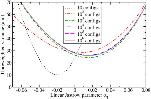
Plots of the unreweighted variance against the value of one of the linear parameters are shown for an all-electron neon atom in Fig. 1. It can be seen that the unreweighted variance converges to a limit as the number of configurations is increased. There is only one minimum in every case.

Figure 1: The unreweighted variance $\sigma_{u}^{2}$ for an all-electron neon atom plotted against one of the linear Jastrow parameters. All of the other linear parameters are set to zero. Different numbers of configurations were used to calculate the quartic coefficients of the unreweighted variance. In each case the configurations were distributed according to the square of the Hartree-Fock wave function. The Jastrow factor contained a total of 24 linear parameters. The curves for $10^{5}$ and $10^{6}$ configurations are indistinguishable in the figure.

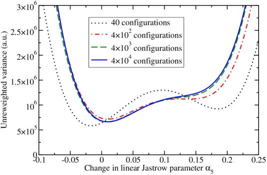
Plots of the unreweighted variance for an all-electron neon atom against the value of a parameter for an extremely poor sampling of configuration space are shown in Fig. 2. When few configurations were used ($N_{C}=40$), it was possible to find two minima of the variance along lines in parameter space, proving that nonglobal minima can exist. However, it was also found that increasing the number of configurations tended to prevent the occurrence of two minima along lines in parameter space.

Figure 2: The unreweighted variance $\sigma_{u}^{2}$ for an all-electron neon atom plotted against the change in one of the linear Jastrow parameters. All the parameters in the Jastrow parameter are set to large, random values. Different numbers of VMC-generated configurations were used to calculate the quartic coefficients of the unreweighted variance. In each case the configurations were distributed according to the square of a Slater-Jastrow wave function, where the Jastrow factor contained the random parameters, so that the resulting distribution was very unlike the ground-state distribution. The Jastrow factor contained a total of 72 linear parameters. The Slater wave function contained Hartree-Fock orbitals.

IV.2 Nonlinear Jastrow parameters

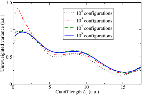
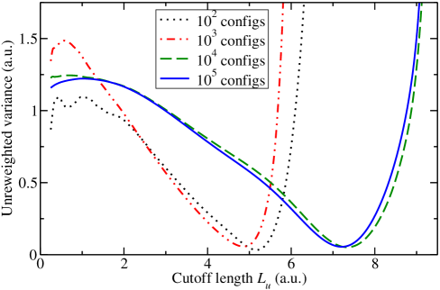
Plots of the unreweighted variance of the SiH₄ molecule against a nonlinear Jastrow parameter—the cutoff length for the electron-electron correlation termndd_jastrow —are shown in Figs. 3 and 4. The behavior of the unreweighted variance is far worse when the cutoff length is varied than when a linear parameter is varied: the variance has multiple minima along lines in parameter space and there is some noise in the variance, especially for poor samplings of configuration space. It can be seen in Fig. 4 that the optimized cutoff lengths obtained using $10^{2}$ or $10^{3}$ configurations are considerably shorter than the cutoff lengths obtained using $10^{4}$ or $10^{5}$ configurations. In the former case the cutoff lengths are trapped in the nonglobal minimum that can be seen in Fig. 3, while the deeper minimum is reached in the latter case. The Jastrow factor used to produce Figs. 3 and 4 is such that the local energy is continuous when an electron-electron separation passes through the cutoff length. If a Jastrow factor that gives rise to a discontinuous local energy at the cutoff length were to be used, the variance would be an extremely noisy function of the cutoff length, especially for thin samplings of configuration space. Optimization of the cutoff lengths for such Jastrow factors has been found to be very difficult.ndd_jastrow The existence of multiple minima when cutoff lengths are optimized suggests that it may be worthwhile performing variance-minimization calculations using several different initial cutoff lengths.

Figure 3: The unreweighted variance $\sigma_{u}^{2}$ for an SiH₄ molecule (with a Hartree-Fock silicon pseudopotentiallee_thesis ) plotted against the cutoff length for the electron-electron terms in the Jastrow factor, $L_{u}$. The Jastrow factor is such that the local energy is continuous when an electron-electron separation passes through the cutoff length.ndd_jastrow Different numbers of VMC-generated configurations were used to calculate the unreweighted variance. All of the linear Jastrow parameters are set to zero. In each case the configurations were distributed according to the square of the Hartree-Fock wave function. The Jastrow factor contained a total of 56 linear parameters, plus three cutoff lengths.

Figure 4: This figure is the same as Fig. 3, except that all of the parameters in the Jastrow factor (including the cutoff lengths) have been optimized.

V Minima of the variance and the energy

V.1 The reweighted and unreweighted variance

V.1.1 Plots of the reweighted and unreweighted variance

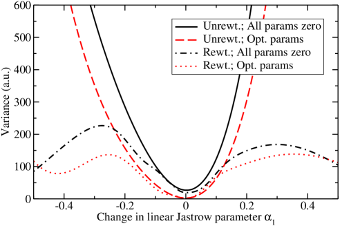
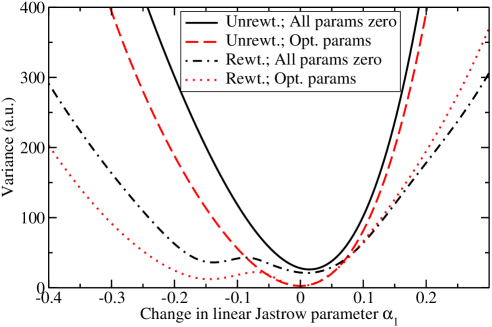
Plots of the reweighted and unreweighted variances for an all-electron neon atom against one of the linear Jastrow parameters are shown in Figs. 5 and 6 for small and large numbers of configurations. The reweighted and unreweighted variances have their minima in different places, with their values at the minima being different from one another. The variance is a smooth function of the linear Jastrow parameter in each case, but there are multiple minima of the reweighted variance along lines in parameter space, demonstrating that nonglobal minima can exist. Furthermore, the minima of the reweighted variance are not as sharply defined as those of the unreweighted variance. Minimization of the unreweighted variance is therefore more likely to be rapid and stable.

Figure 5: The reweighted and unreweighted variance for an all-electron neon atom plotted against the change in the value of a linear Jastrow parameter, $\alpha_{1}$. Plots are shown for the case in which all the parameters are set to zero and the case in which all the parameters have been optimized. The set of 100 configurations used to calculate the variance were distributed according to the square of the Hartree-Fock wave function. The Jastrow factor contained a total of 27 linear parameters.

Figure 6: This figure is the same as Figure 5 except that $10^{4}$ configurations were used to calculate the variance.

V.1.2 Quality of variance-minimization results

The outcomes of reweighted and unreweighted variance-minimization calculations are shown in Table 1. For a relatively sparse sampling of configuration space, reweighted variance minimization is pathologically unstable, while unreweighted variance minimization is perfectly well-behaved. For a dense sampling of configuration space the two methods give very similar results, and there is no evidence that the reweighted variance-minimization algorithm performs any better than the unreweighted algorithm, or vice versa.

			VMC energy (a.u.)				Variance (a.u.)
$P$	$N_{C}$	Cycle	Unrew.		Rew.		Unrew.		Rew.
1	500	1	$-128$.	$5469(5)$	$-128$.	$5469(5)$	$29$.	$3(1)$	$29$.	$3(1)$
1	500	2	$-128$.	$5424(3)$	$-128$.	$5858(3)$	$6$.	$3786(7)$	$6$.	$220(2)$
1	500	3	$-128$.	$6178(3)$	$-128$.	$6129(3)$	$6$.	$310(1)$	$6$.	$207(1)$
1	500	4	$-128$.	$6267(3)$	$-86$.	$508(3)$	$6$.	$1564(7)$	$1501$.	$1(2)$
1	$5\times 10^{5}$	2	$-128$.	$6170(3)$	$-128$.	$6248(3)$	$6$.	$116(2)$	$6$.	$0848(9)$
1	$5\times 10^{5}$	3	$-128$.	$6226(3)$	$-128$.	$6261(3)$	$6$.	$096(1)$	$6$.	$0844(8)$
1	$5\times 10^{5}$	4	$-128$.	$6201(3)$	$-128$.	$6260(3)$	$6$.	$103(1)$	$6$.	$0834(9)$
72	500	2	$-128$.	$87184(9)$	$-128$.	$86664(9)$	$1$.	$4178(7)$	$1$.	$3733(8)$
72	500	3	$-128$.	$88040(9)$	$-50$.	$00(9)$	$1$.	$358(1)$	$420$.	$7(86)$
72	500	4	$-128$.	$8749(1)$	$258$.	$83(1)$	$1$.	$421(2)$	$13599$.	$1(4816)$
72	$5\times 10^{5}$	2	$-128$.	$89760(7)$	$-128$.	$89622(7)$	$1$.	$136(1)$	$1$.	$1330(9)$
72	$5\times 10^{5}$	3	$-128$.	$89742(7)$	$-128$.	$89677(7)$	$1$.	$1343(7)$	$1$.	$132(1)$
72	$5\times 10^{5}$	4	$-128$.	$89752(7)$	$-128$.	$89655(7)$	$1$.	$137(2)$	$1$.	$1326(9)$

Table 1: Results of reweighted and unreweighted variance-minimization calculations for an all-electron neon atom. $P$ is the number of linear parameters in the Jastrow factor and $N_{C}$ is the number of configurations used to perform the optimization. (Long VMC runs were used to obtain the energies and variances shown in the table.) Only linear Jastrow parameters were optimized. The VMC energy and variance for cycle 1 are estimates of the Hartree-Fock energy and variance, and are the same for each $P$ and $N_{C}$.

V.2 Coincidence of the minima of the energy and the variance

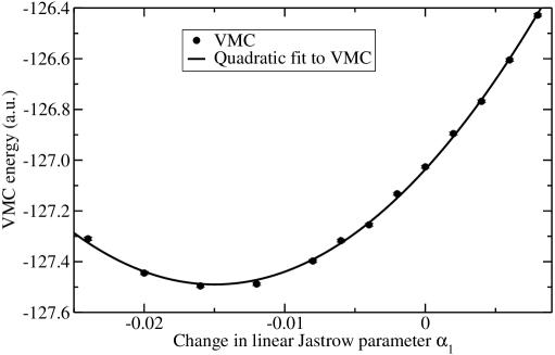
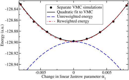
As is clearly demonstrated in Fig. 7, the self-consistent minimum of the unreweighted variance does not necessarily coincide with the minimum of the VMC energy. On the other hand, for a high-quality Jastrow factor, the minima of the unreweighted variance and energy are generally in close agreement, as is shown in Fig. 8. We have no evidence, for all-electron atoms at least, that any significant advantage could be obtained by optimizing linear Jastrow parameters in a good Jastrow factor using an energy-minimization method. It can also be seen in Fig. 8 that the reweighted energy follows the actual VMC energy data closely (the statistical error in the reweighted energy at the optimal wave function is $0.001$ a.u.). This implies that, provided enough configurations are used, the wave function could be optimized by reweighted energy minimization.

Figure 7: The VMC energy against the change in the value of a linear Jastrow parameter $\alpha_{1}$ from the value determined by self-consistent unreweighted variance minimization. The Jastrow factor was chosen to be poor, with no electron-nucleus or electron-electron-nucleus terms, and the same electron-electron terms were used for both parallel and antiparallel spins. There is only one optimizable parameter: $\alpha_{1}$.

Figure 8: The VMC energy of an all-electron neon atom against the change in the value of a linear Jastrow parameter $\alpha_{1}$ from the value determined by self-consistent unreweighted variance minimization. Specifically, the Jastrow factor was the best all-electron neon Jastrow factor described in Ref. ndd_jastrow . The reweighted and unreweighted energies calculated using $8\times 10^{5}$ configurations distributed according to the square of the optimized wave function are also plotted. The statistical error bars in the VMC data are smaller than the symbols.

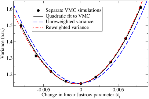
A plot of the VMC energy variance against the change in a linear Jastrow parameter from its optimal value in an all-electron neon atom is shown in Fig. 9. As one would expect, the reweighted variance matches the actual variance, unlike the unreweighted variance; however, there is no significant difference between the minima of the variance and the unreweighted variance (and hence the energy).

Figure 9: The VMC variance for an all-electron neon atom against the change in the value of a linear Jastrow parameter $\alpha_{1}$ from its value determined by self-consistent unreweighted variance minimization. Specifically, the Jastrow factor was the best all-electron neon Jastrow factor described in Ref. ndd_jastrow The reweighted and unreweighted variances calculated using $8\times 10^{5}$ configurations distributed according to the square of the optimized wave function are also plotted. Where the error bars in the VMC data cannot be seen, they are smaller than the symbols.

We have also studied the question of the coincidence of the minima of the energy, the variance, and the self-consistent unreweighted variance using a variety of model systems, for which the integrals could be performed exactly. The models consisted of one-dimensional potential wells and various trial wave functions with a single variable parameter. We studied several examples for a single particle and an example for two identical, interacting fermions. These examples showed that the global minima of the energy, the variance and the self-consistent unreweighted variance can be different. In all cases studied the parameters optimized by self-consistent unreweighted variance minimization gave lower energies than the parameters optimized by reweighted or “true” variance minimization. Furthermore, in many cases, the parameters from the self-consistent unreweighted variance minimum coincided exactly with the energy-minimized parameters, suggesting that some underlying principle was at work.

VI The sampling of configuration space

VI.1 The number of configurations

The VMC energy for a neon-atom Slater-Jastrow wave function is plotted against the number of configurations used to optimize the Jastrow factor in Fig. 10. It can be seen that the wave-function quality improves very rapidly, then saturates at between $5\times 10^{2}$ and $10^{4}$ configurations, for both small and large numbers of parameters. For very small numbers of configurations, the optimizations give pathological results, especially when the more flexible Jastrow factor is used.

Figure 10: The VMC energy of an all-electron neon atom against the number of configurations used to optimize the linear Jastrow parameters in an unreweighted variance minimization. Eight optimization cycles were performed for each number of configurations in order to ensure that self-consistency was achieved. The Slater wave function contained Hartree-Fock orbitals. The error bars in the VMC data are smaller than the symbols.

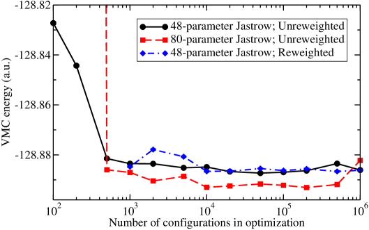
Results obtained using reweighted variance minimization are also shown in Fig. 10. The reweighted variance-minimization process was pathologically unstable for fewer than about $10^{3}$ configurations. For larger numbers of configurations the energies obtained are in good agreement with the results of unreweighted variance minimization.

VI.2 The distribution of configurations

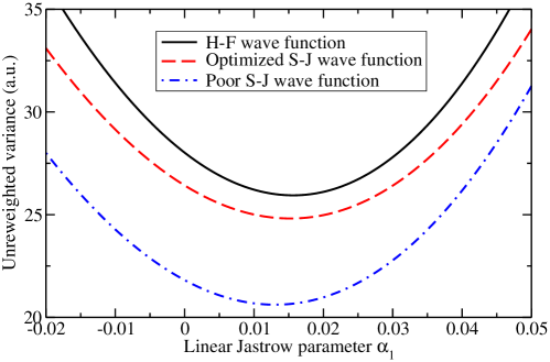
The unreweighted variance for an all-electron neon atom is plotted against a linear Jastrow parameter for three different configuration distributions in Fig. 11. The configurations were distributed according to (i) the square of the Hartree-Fock wave function, as is usually the case in the first cycle of a variance-minimization calculation; (ii) the square of an optimized Slater-Jastrow wave function, as is usually the case in the second and subsequent cycles; and (iii) the square of a Slater-Jastrow wave function in which the Jastrow factor was chosen to be poor. Although the variance looks different in each case, the positions of the minima coincide almost exactly for the Slater and optimized Slater-Jastrow distributions. Even for the poor wave function, the minimum of the variance is reasonably close to the more accurately determined optimum. This is consistent with our observation that, in general, the only significant improvement to the quality of a Jastrow factor occurs in the first cycle of a series of unreweighted variance-minimization calculations: starting from the Hartree-Fock wave function, the self-consistent solution is usually reached in the first cycle.

Figure 11: The unreweighted variance for an all-electron neon atom plotted against the value of the linear Jastrow parameter $\alpha_{1}$ for three different configuration distributions: the square of the Hartree-Fock wave function, the square of an optimized Slater-Jastrow wave function and the square of a poor Slater-Jastrow wave function. $10^{6}$ configurations were used to calculate the unreweighted variance. The Jastrow factor contained a total of 36 linear parameters. The Slater wave function contained Hartree-Fock orbitals.

VII The flexibility of the Jastrow factor

The VMC energy of neon is plotted against the number of linear parameters used in the Jastrow factor in Fig. 12. The results illustrate the futility of attempting to optimize too many parameters. The quality of the optimized wave function depends on the number of configurations used to perform the optimization, especially when the number of parameters in the wave function is either very small or very large. However, there would only appear to be an advantage to be gained by using more than $10^{4}$ configurations when a very large number of parameters are to be optimized.

Figure 12: The VMC energy of an all-electron neon atom against the number of parameters in the Jastrow factor. Different numbers of configurations were used to carry out the unreweighted variance-minimization calculations. Six optimization cycles were performed in order to guarantee self-consistency. Very long VMC simulations were carried out using the optimized Jastrow factors in order to obtain the energies plotted in the graph. The VMC error bars are smaller than the symbols. The Slater wave function contained Hartree-Fock orbitals.

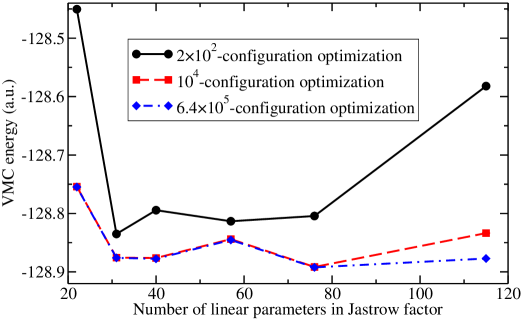
It should be reemphasized that the problems which occur when large numbers of parameters are optimized are caused by mismatches between the minima of the unreweighted variance and the energy, and not by the introduction of local minima into the variance landscape.

VIII Limiting of configuration weights

It has been suggested that variance-minimization calculations are disproportionately affected by “outlying” configurations, whose energies deviate substantially from the mean energy.kent_1999 In particular, the local energy diverges in the vicinity of the nodal surface of the trial wave function, so configurations in this region are especially problematic. Such configurations are relatively rare when the nodes are fixed, as is the case when only Jastrow parameters are optimized, but the problem can be far more serious when parameters that affect the nodal surface are optimized using a fixed sampling of configuration space.

We have studied a smooth scheme for removing outlying configurations from the optimization process. Let us define the configuration “effective weight” to be

$$W^{\prime}({\bf R})=\frac{1}{2}\left[1-\tanh\left(\frac{\left(E_{L}^{\{\alpha\}}({\bf R})-\bar{E}_{u}\right)^{2}-A^{2}\sigma^{2}_{u}}{B^{2}\sigma^{2}_{u}}\right)\right],$$ (44)

where $\bar{E}_{u}$ and $\sigma^{2}_{u}$ are the unreweighted energy and variance of the set of configurations. $W^{\prime}({\bf R})\approx 1$ for configurations such that $E_{L}^{\{\alpha\}}({\bf R})\approx\bar{E}_{u}$, but $W^{\prime}({\bf R})\rightarrow 0$ for configurations whose local energies are far from the mean. The parameter $A$ is the number of standard deviations of the energy beyond which configurations are excluded, while $B$ is the width of the region in which the effective weights fall off to zero (in terms of standard deviations of the energy). We typically chose $A$ to lie between 2 and 3 and $B$ to lie between $1/2$ and $1$. The effective weights $W^{\prime}$ are used in place of the weights $W$ in Eq. (4), and the reweighted variance $\sigma_{w}^{2}$ is minimized.

We have found that this weight-limiting scheme is capable of improving the stability of Jastrow-factor optimization when very small numbers of configurations are used. However, the energies of the resulting wave functions are not generally as good as the energies obtained using the same forms of wave function optimized with an adequate number of configurations. For large numbers of configurations, the limiting scheme has very little effect on the optimization of Jastrow factors. We conclude that the weight-limiting scheme is not of much practical benefit when a Jastrow factor is to be optimized; however the scheme has been found to be very useful when parameters that affect the nodal surface are optimized.plr_comm

Other limiting schemes have been devised to improve the stability of the variance-minimization algorithms. For example, it is possible to combine the reweighted and unreweighted variance-minimization algorithms by limiting the values that the weights $W$ can take.filippi_1996 Alternatively, the local energies themselves can be limited.kent_1999 The latter approach has been found to be problematic, as it can result in spurious minima in the variance corresponding to parameter sets for which a large number of local energies are limited.

IX Scaling of the variance-minimization methods

IX.1 CPU time required for the optimization phase

Let $N$ be the total number of electrons in a system, $P$ be the number of Jastrow parameters to be optimized, and $N_{C}$ be the number of configurations used to calculate the variance. Although the Jastrow factor of Ref. ndd_jastrow is considered in this work, the conclusions reached should be valid for most other forms of Jastrow factor in current use.

The computational effort required to evaluate the unreweighted variance using the accelerated method is independent of $N$ and $N_{C}$, but scales as $O(P^{4})$. The time taken to compute the gradient of the variance is also $O(P^{4})$. It may be assumed that the number of optimization steps required is independent of $P$, $N$, and $N_{C}$. The $O(P^{4})$ scaling of the memory requirements of the accelerated method limits the number of parameters that can be optimized in a single calculation to between 100 and 200, depending on the available memory.

The time taken to recompute the Jastrow factor and its derivatives after all of the parameters have changed is generally $O(N)$ for electron-nucleus and electron-electron-nucleus terms and $O(N^{2})$ for electron-electron terms.ndd_jastrow The CPU time required to evaluate the variance (reweighted or unreweighted) using the standard procedure therefore increases as $O(N^{2})$. The time taken to calculate the Jastrow factor is, in general, $O(P)$, and hence the time taken to calculate the variance using the standard method is also $O(P)$. Furthermore, each minimization step requires the gradient of the variance with respect to the parameters, which has $P$ components The time taken to perform each iteration is therefore $O(P^{2})$. The CPU time for the standard method clearly scales as $O(N_{C})$.

Putting this together, the CPU time for the optimization phase scales as $O(P^{4})$ for the accelerated method and $O(N^{2}P^{2}N_{C})$ for the standard method. It should be noted that the time required by the optimization phase in the accelerated scheme is completely negligible in comparison with the time required by the VMC coefficient-gathering phase, whereas the CPU time required by the optimization phase in the standard method is usually rather greater than the CPU time required by the VMC phase.

IX.2 The CPU time required for the gathering of the quartic coefficients in the accelerated scheme

In the standard variance-minimization method, the CPU time required to generate the set of configurations used to compute the variance does not differ appreciably from the time taken to perform an ordinary VMC simulation. For the accelerated optimization method, however, the time taken to compute the quartic expansion coefficients can be a significant fraction of the total CPU time.

The gathering of the quartic coefficients can be divided into two stages: (i) the evaluation of the Jastrow “basis functions” $f_{i}({\bf R})$ for each configuration ${\bf R}$ (see Eq. (11)), and (ii) the calculation of the corresponding contributions to the $\bar{g}$ and $\bar{G}$ arrays. Stage (ii) scales as $O(P^{4})$, but is independent of system size. By contrast, stage (i) scales as $O(P)$, because there are $P$ basis functions, but the scaling with system size is the same as that of evaluating the Jastrow factor: roughly $O(N^{2})$.

The CPU time for an ordinary VMC calculation is generally determined by the time taken to evaluate the orbitals in the Slater wave function. The computational effort required to carry out a fixed number of configuration moves grows as $O(N^{2})$ if extended orbitals represented in a localized basis are used. The use of localized orbitals can improve this scaling to $O(N)$.williamson_lin_scaling In principle the time taken for stage (i) of the coefficient gathering will take up an increasingly large fraction of the CPU time, but in practice the prefactor is so small that the time required is negligible even for the largest systems that we have studied. The time taken for stage (ii) can be the largest contribution to the CPU time for VMC simulations of small molecules, but the effort required is independent of system size, and so, overall, the coefficient-gathering phase of the accelerated scheme is more efficient for large systems than small systems.

X Efficiency of the accelerated optimization method

Timing results for the optimization of the linear Jastrow parameters for an H₂O molecule (10 electrons) and a C₂₆H₃₂ molecule (136 electrons) are shown in Tables 2 and 3 respectively. The calculations are fairly typical in terms of the number of parameters and number of configurations. In both cases the use of the accelerated optimization scheme essentially eliminates the cost of the optimization phase. In the standard method the cost of the optimization phase exceeds that of the VMC configuration-generation phase by an order of magnitude for H₂O and by a less significant proportion for C₂₆H₃₂. The cost of the VMC phase in the accelerated scheme is increased substantially for H₂O although, overall, it is still much faster to use the accelerated scheme. For C₂₆H₃₂ the increase in the CPU time for configuration generation is negligible. Overall, the accelerated optimization scheme is 4.5 times faster for H₂O and 2.3 times faster for C₂₆H₃₂.

Method	Stage	CPU time (s)
	VMC	$5669$.	$43$
Standard	Opt.	$58740$.	$65$
	Total	$64410$.	$08$
	VMC	$14378$.	$90$
Accel.	Opt.	$39$.	$69$
	Total	$14418$.	$59$

Table 2: Timing results for ten cycles of a $6\times 10^{4}$-configuration unreweighted variance minimization of a 38-linear-parameter Jastrow factor for an all-electron H₂O molecule. The system contains a total of 10 electrons. The Slater wave function contained Hartree-Fock orbitals. The runs were carried out on a 1.7 GHz Pentium processor in a Sony Vaio laptop.

Method	Stage	CPU time (s)
	VMC	$6526$.	$77$
Standard	Opt.	$9323$.	$53$
	Total	$15850$.	$30$
	VMC	$6828$.	$47$
Accel.	Opt.	$28$.	$14$
	Total	$6856$.	$61$

Table 3: Timing results for four cycles of a $1.6\times 10^{4}$-configuration unreweighted variance minimization of a 12-linear-parameter Jastrow factor for a C₂₆H₃₂ molecule with Troullier-Martins carbon and hydrogen pseudopotentials. The system contains a total of 136 electrons. The Slater wave function contained DFT-PBE orbitals. The runs were carried out on a cluster of eight 2.1 GHz Opteron processors.

The actual time taken to compute the variance in the accelerated scheme is minute: On a 2.7 GHz Pentium 4 processor, it takes an average of $83.6$ $\mu$s to compute the variance with 25 parameters, while it takes $13.98$ ms to compute the variance with 100 parameters.

XI Conclusions

We have introduced a new scheme for evaluating the unreweighted variance of the VMC energy, which greatly accelerates the optimization of parameters that occur in a linear fashion in the exponent of a Jastrow factor. This scheme is very efficient because it uses the property that the unreweighted variance is a quartic function of such parameters. We studied a wide range of systems and found that the unreweighted variance almost invariably has a single minimum in the space of the linear parameters. The only exceptions to this that we could find occurred when the configuration space was very poorly sampled. For other wave-function parameters, however, the unreweighted variance often has more than one minimum.

It is easy to use very large numbers of configurations to perform optimizations using our accelerated scheme. We have investigated the effect of varying the number of configurations on the wave-function quality, and we have found that there is, in general, no significant benefit to be obtained from using more than about $10^{4}$ configurations when optimizing linear Jastrow parameters.

We have considered various wave-function optimization schemes using correlated-sampling approaches for minimizing the energy and the variance of the energy. Reweighted energy and variance minimization using correlated sampling suffer from numerical instabilities due to fluctuations in the values of the weights, which are severe for large systems. The unreweighted energy always has a stationary point at the wave function used to generate the configuration set, and for parameters which occur linearly in the Jastrow factor this stationary point is the global maximum in the energy. The unreweighted energy is therefore not a suitable cost function for wave-function optimization. The minima of the variance, the unreweighted variance (iterated to self-consistency), and the energy are generally distinct. In various model systems that we have studied, the self-consistent minimum in the unreweighted variance always gave lower energies than the minimum in the reweighted variance.

XII Acknowledgments

Financial support was provided by the Engineering and Physical Sciences Research Council (EPSRC), UK. Computing resources have been provided by the Cambridge-Cranfield High Performance Computing Facility.

Appendix A Constructing the quartic polynomial corresponding to a line in parameter space

Consider the expression for the quartic unreweighted variance as a function of the linear parameters (Eq. (34)), and consider a line in parameter space

$$\mbox{\boldmath$\alpha$}(t)={\bf A}+{\bf B}t,$$ (45)

where $\mbox{\boldmath$\alpha$}=(\alpha_{1},\ldots,\alpha_{P})$ and ${\bf A}$ and ${\bf B}$ are constant vectors. The unreweighted variance along the line is given by

$$\sigma_{u}^{2}(t)=\frac{N_{C}}{N_{C}-1}\left(\Omega_{4}t^{4}+\Omega_{3}t^{3}+\Omega_{2}t^{2}+\Omega_{1}t+\Omega_{0}\right),$$ (46)

where

$$\Omega_{4} = \sum_{i=1}^{P}B_{i}\sum_{j=i}^{P}B_{j}\sum_{k=j}^{P}B_{k}\sum_{l=k}^{P}B_{l}\Gamma_{ijkl}^{(4)}$$ (47)

$$\Omega_{3} = \sum_{i=1}^{P}A_{i}\sum_{j=i}^{P}B_{j}\sum_{k=j}^{P}B_{k}\sum_{l=k}^{P}B_{l}\Gamma_{ijkl}^{(4)}+\sum_{i=1}^{P}B_{i}\sum_{j=i}^{P}A_{j}\sum_{k=j}^{P}B_{k}\sum_{l=k}^{P}B_{l}\Gamma_{ijkl}^{(4)}$$ (48)

$${}+\sum_{i=1}^{P}B_{i}\sum_{j=i}^{P}B_{j}\sum_{k=j}^{P}A_{k}\sum_{l=k}^{P}B_{l}\Gamma_{ijkl}^{(4)}+\sum_{i=1}^{P}B_{i}\sum_{j=i}^{P}B_{j}\sum_{k=j}^{P}B_{k}\left(\Gamma_{ijk}^{(3)}+\sum_{l=k}^{P}A_{l}\Gamma_{ijkl}^{(4)}\right)$$

$$\Omega_{2} = \sum_{i=1}^{P}A_{i}\sum_{j=i}^{P}A_{j}\sum_{k=j}^{P}B_{k}\sum_{l=k}^{P}B_{l}\Gamma_{ijkl}^{(4)}+\sum_{i=1}^{P}A_{i}\sum_{j=i}^{P}B_{j}\sum_{k=j}^{P}A_{k}\sum_{l=k}^{P}B_{l}\Gamma_{ijkl}^{(4)}$$ (49)

$${}+\sum_{i=1}^{P}A_{i}\sum_{j=i}^{P}B_{j}\sum_{k=j}^{P}B_{k}\left(\Gamma_{ijk}^{(3)}+\sum_{l=k}^{P}A_{l}\Gamma_{ijkl}^{(4)}\right)+\sum_{i=1}^{P}B_{i}\sum_{j=i}^{P}A_{j}\sum_{k=j}^{P}A_{k}\sum_{l=k}^{P}B_{l}\Gamma_{ijkl}^{(4)}$$

$${}+\sum_{i=1}^{P}B_{i}\sum_{j=i}^{P}A_{j}\sum_{k=j}^{P}B_{k}\left(\Gamma_{ijk}^{(3)}+\sum_{l=k}^{P}A_{l}\Gamma_{ijkl}^{(4)}\right)$$

$${}+\sum_{i=1}^{P}B_{i}\sum_{j=i}^{P}B_{j}\left(\Gamma_{ij}^{(2)}+\sum_{k=j}^{P}A_{k}\left(\Gamma_{ijk}^{(3)}+\sum_{l=k}^{P}A_{l}\Gamma_{ijkl}^{(4)}\right)\right)$$

$$\Omega_{1} = \sum_{i=1}^{P}B_{i}\left(\Gamma_{i}^{(1)}+\sum_{j=i}^{P}A_{j}\left(\Gamma_{ij}^{(2)}+\sum_{k=j}^{P}A_{k}\left(\Gamma_{ijk}^{(3)}+\sum_{l=k}^{P}A_{l}\Gamma_{ijkl}^{(4)}\right)\right)\right)$$ (50)

$${}+\sum_{i=1}^{P}A_{i}\sum_{j=i}^{P}B_{j}\left(\Gamma_{ij}^{(2)}+\sum_{k=j}^{P}A_{k}\left(\Gamma_{ijk}^{(3)}+\sum_{l=k}^{P}A_{l}\Gamma_{ijkl}^{(4)}\right)\right)$$

$${}+\sum_{i=1}^{P}A_{i}\sum_{j=i}^{P}A_{j}\sum_{k=j}^{P}B_{k}\left(\Gamma_{ijk}^{(3)}+\sum_{l=k}^{P}A_{l}\Gamma_{ijkl}^{(4)}\right)+\sum_{i=1}^{P}A_{i}\sum_{j=i}^{P}A_{j}\sum_{k=j}^{P}A_{k}\sum_{l=k}^{P}B_{l}\Gamma_{ijkl}^{(4)}$$

$$\Omega_{0} = \Gamma^{(0)}+\sum_{i=1}^{P}A_{i}\left(\Gamma_{i}^{(1)}+\sum_{j=i}^{P}A_{j}\left(\Gamma_{ij}^{(2)}+\sum_{k=j}^{P}A_{k}\left(\Gamma_{ijk}^{(3)}+\sum_{l=k}^{P}A_{l}\Gamma_{ijkl}^{(4)}\right)\right)\right).$$ (51)

All the terms that appear in Eqs. (47)–(51) can be evaluated within a single loop over $i$, $j$, $k$, and $l$.

References

- (1) W. M. C. Foulkes, L. Mitas, R. J. Needs, and G. Rajagopal, Rev. Mod. Phys. 73, 33 (2001).
- (2) C. J. Umrigar, K. G. Wilson, and J. W. Wilkins, Phys. Rev. Lett. 60, 1719 (1988).
- (3) P. R. C. Kent, R. J. Needs, and G. Rajagopal, Phys. Rev. B 59, 12344 (1999).
- (4) R. J. Needs, M. D. Towler, N. D. Drummond, and P. R. C. Kent, casino version 1.7 User Manual, University of Cambridge, Cambridge (2003).
- (5) In Ref. kent_1999 it was stated that the unreweighted energy could have a maximum, minimum, or saddle point at the parameter values , but this is incorrect; we have proved that it is always a maximum.
- (6) N. D. Drummond, M. D. Towler, and R. J. Needs, Phys. Rev. B 70, 235119 (2004).
- (7) W. H. Press, S. A. Teukolsky, W. T. Vetterling, and B. P. Flannery, Numerical Recipes in Fortran 77 (2nd ed.), Cambridge University Press (1992).
- (8) Y. Lee, PhD Thesis, University of Cambridge, Cambridge (2002).
- (9) P. Lopez Rios, Personal communication (2005).
- (10) C. Filippi and C. J. Umrigar, J. Chem. Phys. 105, 213 (1996).
- (11) A. J. Williamson, R. Q. Hood, and J. C. Grossman, Phys. Rev. Lett. 87, 246406 (2001).