Complex patterns and tip effect evolution

Abstract

We studied the formation of complex patterns using a variational principle and a standard energy functional. These patterns evolve by letting the system to search for the optimal configuration of a high conductivity channel, that in one dimension is equivalent to tip effect evolution (evolution towards regions of high electric field).

The similarities between complex patterns produced spontaneously in dielectric breakdownuman ; dbm84 ; dbm95 , snowcrystalslanger ; rmp93 ; jacob93 , viscous fingersbensimon ; mccloud , etc., is suggestive for the existence of an universal explanation for their appearance, the lack of a general model that explains the appearance of these patterns and the apparent difficulty of this subject, leads to the common belief that no simple general principle can explain this diversity of complex patterns.

Some years ago we started the search for an universal energy functional from which complex patterns should appear. After simplifying the typical dynamical equations for several systems, elimination of microscopic details, and neglecting time dependent variables, we were left with a simple Laplace equationsaarlos .

The most general form of Laplace equation includes a conductivity that depends on spatial coordinates, it turns out that in our model this conductivity will have different values inside the pattern and in the region outside the pattern. Laplace equation is a good starting point, because this equation is a consequence of a conservation law for the flux of the vectorial field. It is well known that Laplace equation can be obtained from a variational principle, and the energy functional can be found in any textbook of electromagnetism. We found that this energy functional can produce a great variety of complex patterns, when used in a quasi-static model that let the system to probe different configurations for the conductivity and evolve towards the one where the energy functional is maximized.

In this work we studied charged capacitors that are in a static configuration for the scalar field, but not in a state of minimal energy. For high voltages, the dielectric is able to increase locally the permittivity and a conducting channel can be formed between boundaries. This would allow the system to equalize the values for the scalar field at the boundaries, releasing the stored energy. Tip effect and screening are essential effects in the study of these systems, we understand our model as a generalization of tip effect evolution: instead of evolving the channel towards the regions of high electric field, we evolve the channel towards regions that maximize the energy functional. Tip effect evolution and our model are equivalent for one-dimensional systems, but for higher dimensions our model can produce complex patterns. Other models that use tip effect, must include an independent mechanism to produce complex patterns. Using a direct implementation of our model and different numerical algorithms, we have obtained non-trivial results for dielectric breakdown patterns.

To understand the underlying physics, we explain the model using an electric scalar field $\phi$ inside a parallel plate capacitor: After imposing boundary conditions and given the permittivity $\epsilon$, which in general depends on coordinates, one must solve Laplace equation

$$\nabla\cdot(\epsilon\nabla\phi)=0,$$ (1)

to obtain $\phi$ in the region of interest. It is well known that this equation can be derived, using a variational principle, from the energy functional

$$U=\frac{1}{2}\int\epsilon(\nabla\phi)dV.$$ (2)

$U$ is also the total energy in the capacitor when the charge $Q$ is maintained constant. In the case of a parallel plate capacitor this energy will be proportional to $d/\epsilon$, where $d$ is the separation between the plates. Static physical systems evolve trying to reduce the total energy, this implies a force between the plates trying to reduce the distance $d$, and if you insert a slab of a dielectric material having a permittivity $\epsilon$’ greater than $\epsilon$, the slab will be pulled into the capacitor. If instead of maintaining $Q$ constant, the potential difference between the plates $V$ is maintained constant, the energy $U$ for this system will be proportional to $\epsilon/d$. In experiments at constant $Q$ or $V$ there are forces trying to reduce d and to increase $\epsilon$, then in experiments at constant $V$, $U$ is not the total energy of the system, because the system evolves trying to increase $U$. There is a missing energy term coming from a rearrangement of charges in the wires to maintain $V$ constant. When this term is introduced, the total energy is again proportional to $d/\epsilon$. The previous discussion justifies that we study systems at constant $V$ by letting them to evolve towards regions of higher $U$.

If V is large enough the dielectric material will break causing a short circuit, we propose that for large V there is a new possibility for the system to lower the total energy, a short circuit. Assuming that $\epsilon$ can evolve locally towards bigger values, forming a discharge channel, we could obtain complex patterns of permittivity by letting the system to evolve towards higher values of U. Our model is quasi-static (see below), but there are two implicit time scales in the problem: a slow evolution for a local change in $\epsilon$, and a fast evolution for the electric potential $\phi$ after a local change in $\epsilon$. For these systems, complex patterns are produced because the system is trying to lower the total energy by increasing locally the permittivity.

Because the evolution for these systems is highly nonlinear, we have to rely on numerical methods to study the growing of patterns. We study these systems using a quasi-static treatment as follows: First, set the boundary conditions which are maintained trough all the steps in our simulation. Second, assign a fixed value $\epsilon$ to the permittivity inside the boundaries. Third, using Laplace equation, obtain $\phi$ after changing the permittivity locally to a greater value $\epsilon^{\prime}$, near one electrode. Fourth, find the energy U using the new values for the permittivity and the scalar field. Fifth, repeat steps 3 and 4 to obtain the energy values U for each of the neighbors of one electrode. These energies are compared and the neighbor providing the biggest energy value is added to the channel. These steps are repeated including the new neighbors for the channel, until a pattern develops. We used a square lattice, pattern evolution through the diagonals is not permitted, and the pattern grows adding only one site to the evolving pattern at each time step.

The lightning discharge in thunderstormsuman and sparks between charged conductors, evolve forming a branched structure that resembles a fractalmandelbrot . The presently accepted model of lightningdbm84 ; dbm95 was developed by Niemeyer, Pietronero and Wiesmann in 1984. They include a stochastic term that weights a probability, that is a function of the value of the local electric field. This is known as the Dielectric Breakdown Model (DBM) and produces a branched structure whose fractal dimension is similar to the ones obtained experimentally for the same geometry, Pietronero model is based on the Diffusion Limited Aggregation (DLA) model, developed by Witten and Sander in 1981dla .

Our results show that it is possible to obtain a branched structure of lightning that follow from a deterministic treatmentfvera1 , that only relies in minimizing the total energy in the system and local changes in the permittivity of the medium (not the geometry of the inner electrode) at each step of iteration. We note that our model is almost all of the time deterministic, but for some configurations there is degeneracy for the extreme value of the energy $U$, and the numerical noise will be responsible for selecting the next step in the evolution of our simulated patterns.

We studied dielectric breakdown in the circular geometry of Fig. 1, considering a $20\times 20$ two-dimensional square lattice, where the central point is the inner electrode and the outer electrode is modeled as a circle. The boundary conditions, $\phi=0$ in the inner electrode and $\phi=1$ in the outer electrode, are maintained trough all the steps in our simulation. For each different configuration, the numerical solution of Laplace equation was obtained using a Successive Over Relaxation algorithm and accepted when the numerical residual was less than $10^{-2}$, the values for the permittivity outside the channel was $\epsilon=1$ and inside the channel was $\epsilon^{\prime}=5$. The filled boxes represent the discharge channel (sites where the permittivity is $\epsilon^{\prime}$). The circles show all possible sites where the channel can evolve, the diameter of each of these circles represent the value for the energy U of the system if this site is added to the channel.

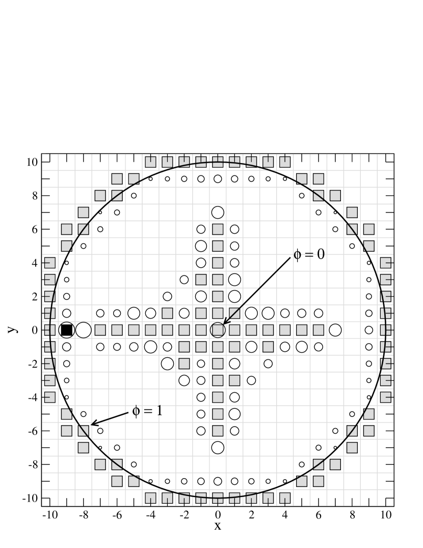
Figure 1: Discharge channel, for a $20\times 20$ square lattice, showing the attachment between the return branch (left black box) and the main branch (inner gray boxes).

Because upward-moving discharges initiated from earth attach with the downward-moving leader in real lightning, we considered two initial branches: the main branch coming from the central lattice site and the return branch coming from the outer electrode. The return branch begin to evolve, after 36 steps of evolution of the main branch, at the site having the black box inside (at the extreme left of the figure). The site between this point and the main branch is the next step in the evolution, completing the path for this discharge channel from the inner electrode towards the outer electrode. The return branch obtained in our numerical simulations is a highly non trivial result and we do not know of any other work that can obtain this attachment.

Fig. 2 shows the structure of the pattern evolved from the central lattice site for a $70\times 70$ square lattice after 750 iterations. For each different configuration, the numerical solution of Eq. 1 was obtained using a Successive Over Relaxation algorithm and accepted when the numerical residual was less than $10^{-1}$, the values for the permittivity outside the channel was $\epsilon=2$ and inside the channel was $\epsilon^{\prime}=6$. The evolution of the pattern shows that opposite branches are not exactly aligned, it is possible to find this effect in the experimental results for snowcrystal growth shown in Fig. 3 of ref langer . Our example also shows that the system develops forming initially a central compact core, this core supports the evolution of the main venous branches and diagonal branches. We expect that secondary branches, emerging from the main branches, would appear after some additional iterations. Because we are using a direct implementation of the principle of least action, that is nicely explained in the textbook of Richard Feynmanfeynman , we solve Laplace equation for a permittivity change of each neighbor, assigning permanently the value $\epsilon^{\prime}$ only to the neighbor with biggest U. This procedure is very time consuming and several months of computing time was needed for completing this example.

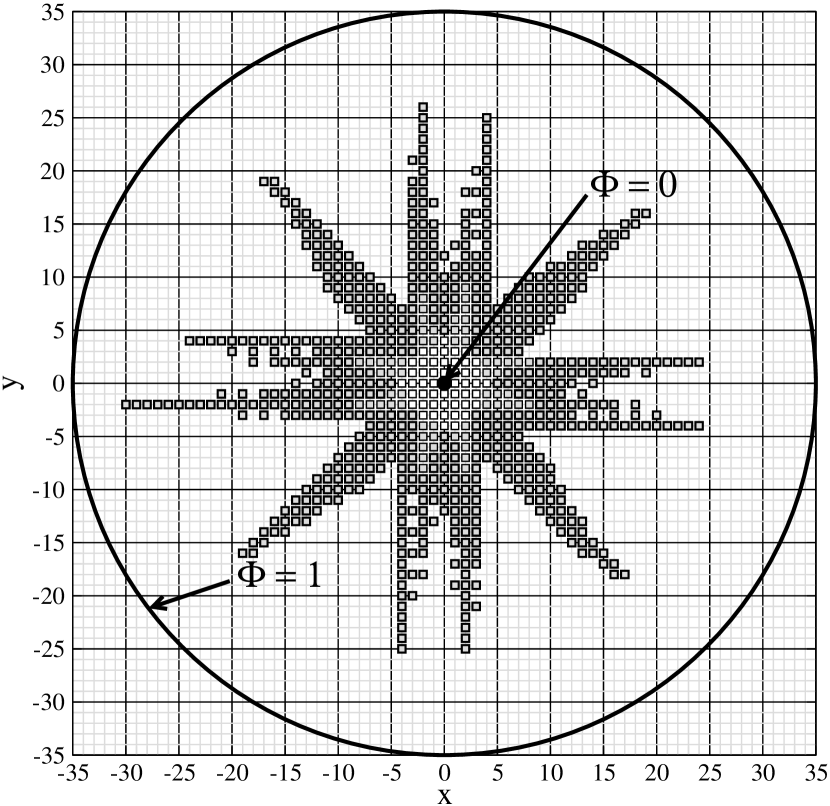
Figure 2: Pattern developed for a $70\times 70$ square lattice, started at the central site, after 750 iterations, for $\epsilon=2$ outside the channel and $\epsilon^{\prime}=6$ inside the channel.

To reduce the computing time needed for obtaining patterns, we have re-implemented our model using adaptive grid algorithmsmitchell . We used two grids to study the evolution of patterns: a square lattice to evolve the pattern and an adaptive grid based on triangles to solve Laplace equation. The adaptive grid algorithms implemented, pose the additional restriction of solving Laplace equation in rectangular domains. We forced the circular geometry (1/4 of a circle) by solving the equations in the unit square, setting the permittivity to very high values ($\epsilon=1000$), when $x^{2}+y^{2}\geq 1$ and the following boundary conditions: $\phi=1$ at the top and right boundaries, $\phi=0$ at the origin (0,0), $\phi=x$ at the bottom, and $\phi=y$ at the left boundary.

We studied the evolution of a pattern starting from the origin using a $100\times 100$ square lattice, 20000 nodes for the adaptive grid, $\epsilon=1$, and $\epsilon^{\prime}=3$. For this sector of a circle, the pattern begin to grow following the diagonal in a way similar to the diagonal branches of fig. 2, after 13 steps this branch begin to depart from the diagonal. As the number of neighbors increases, this calculation begins to slow down.

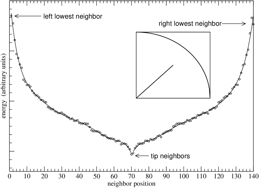
Figure 3: Energy U as a function of neighbor position for a diagonal of length 70 starting at (0,0), in a sector of a circular domain as shown in the inset. The calculation was done in a $100\times 100$ square lattice, using 20000 nodes for the adaptive grid, $\epsilon=1$, and $\epsilon^{\prime}=3$.

To gain some insight, we have carried out calculations of the energies U for the neighbors of a given fixed pattern. We forced a one-dimensional line of permittivity $\epsilon^{\prime}$ and length 70 along the diagonal, starting at (0,0), as shown in the inset of figure 3. In this figure we plot the energies U obtained after a local change of each neighbor permittivity towards $\epsilon^{\prime}$, neighbors near position 1 correspond to the line left lowest neighbors, neighbors near position 70 correspond to the line tip neighbors, and neighbors near position 140 correspond to the line right lowest neighbors. In this plot we fitted 7th grade polynomials for the left and right branches. Because the system evolves towards high values of U, this line would evolve towards the lowest neighbors and not towards the tip neighbors. This evolution is contrary to tip effect evolution and is a consequence of the finite value $\epsilon^{\prime}$ and geometry.

To investigate the effect of geometry, we studied the evolution of a pattern starting from the central site of the bottom boundary in a unit square domain and the following boundary conditions: $\phi=1$ at the top, $\phi=0$ at the bottom, $\phi=y$ at the left boundary, and $\phi=y$ at the right boundary. Using a $100\times 100$ square lattice to evolve the pattern, 20000 nodes for the adaptive grid, $\epsilon=1$, and $\epsilon^{\prime}=20$, the pattern grows as a vertical one-dimensional line. This is exactly what is expected from tip effect evolution and shows that the numerical error is well controlled in our simulations.

To show the differences between our model and tip effect evolution, we forced a 1-dimensional vertical line of permittivity $\epsilon^{\prime}$ and length 70, starting at the central site of the bottom boundary, as shown in the inset of fig. 4. In this figure, we plot the energies U obtained after a local change of each neighbor permittivity towards $\epsilon^{\prime}$, as a function of neighbor position. We used the same boundary conditions mentioned in the previous paragraph, $\epsilon=1$ and $\epsilon^{\prime}=3$. In this case, a permittivity change in the neighbor just above the tip gives the pattern of highest U, explaining the previous vertical line evolution. This plot provides much more information than just tip effect evolution. If an independent mechanism, like surface tension, is introduced to prevent tip evolution, the left and right lowest neighbors could begin to evolve.

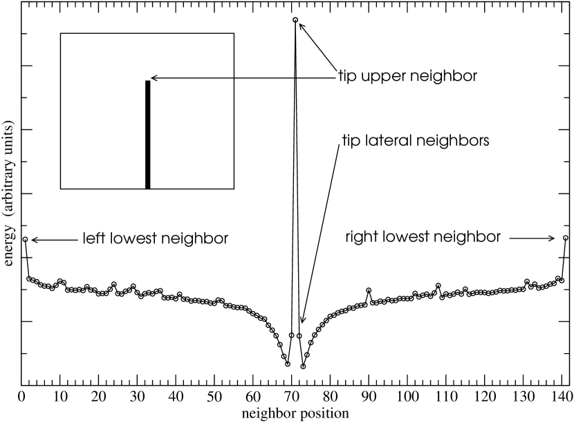
Figure 4: Energy U as a function of neighbor position for a vertical line of length 70 starting at the center of the bottom boundary, in a square domain. The calculation was done in a $100\times 100$ square lattice, using 20000 nodes for the adaptive grid, $\epsilon=1$, and $\epsilon^{\prime}=3$.

To summarize: We have obtained non trivial patterns using a simple and well known energy functional. Contrary to other models, our model is not stochastic and the generated patterns are not of dynamical origin. Our model needs much more computing time than other models in the literature, because the system has to probe different possible configurations and select the one minimizing the total energy. We have seen the appearance of a return branch, which is typically found in real lightning. We obtained the breaking of chiral symmetry in a global pattern, as a consequence of degeneracy and time evolution. In circular geometries, the patterns obtained using our model, show branches that are roughly identical in length, we obtained this very important result straightforward by letting the system to evolve locally towards a configuration of minimal energy. For the same set of parameters we have seen a pattern to grow first in a compact form, and after reaching a critical size the system begin to form branches. For some geometries tip growing is favored, for other geometries the system try to increase the width of the channel. Because the evolving pattern changes the geometry, and the evolution depends on system history, there are many possibilities for complex patterns to appear. In the near future we expect to obtain fractal like structures from our numerical simulations.

We hope that this mechanism of reducing energy by increasing conductivities could be applied to many others different pattern forming systems.

References

- (1) M. A. Uman and E. P. Krider, Science 246, 457 (1989).
- (2) L. Niemeyer, L. Pietronero, and H. J. Wiesmann, Phys. Rev. Lett. 52, 1033 (1984).
- (3) A. Erzan, L. Pietronero, and A. Vespignani, Rev. Mod. Phys. 67, 545 (1995).
- (4) J. S. Langer, Rev. Mod. Phys. 52, 1 (1980).
- (5) E. Ben-Jacob, Contemporary Physics 34, 247 (1993).
- (6) M. C. Cross and P. C. Hohenberg, Rev. Mod. Phys. 65, 851 (1993).
- (7) D. Bensimon, L. Kadanoff, S. Lang, B. Shraiman, and C. Tang, Rev. Mod. Phys. 58, 977 (1986).
- (8) K. McCloud and J. Maher, Physics Reports 260, 139 (1995).
- (9) W. M. Saarloos, Physics Reports 301, 9 (1998).
- (10) B. Mandelbrot, "Fractals: Form, Chance and Dimension" (Freeman, San Francisco, 1977).
- (11) T. A. Witten, L. M. Sander, Phys. Rev. Lett. 47, 1400 (1981).
- (12) F. Vera, http://www.arxiv.org/abs/nlin/0206011 (2002).
- (13) R. P. Feynman, R. B. Leighton, M. Sands, The Feynman lectures on physics (vol. 2, Addison Wesley, 1964).
- (14) W. Mitchell, Proceedings of the 2002 International Conference on Computational Science (2002).