Fluctuations in type IV pilus retraction

Abstract

The type IV pilus retraction motor is found in many important bacterial pathogens. It is the strongest known linear motor protein and is required for bacterial infectivity. We characterize the dynamics of type IV pilus retraction in terms of a stochastic chemical reaction model. We find that a two state model can describe the experimental force velocity relation and qualitative dependence of ATP concentration. The results indicate that the dynamics is limited by an ATP-dependent step at low load and a force-dependent step at high load, and that at least one step is effectively irreversible in the measured range of forces. The irreversible nature of the sub-step(s) lead to interesting predictions for future experiments: We find different parameterizations with mathematically identical force velocity relations but different fluctuations (diffusion constant). We also find a longer elementary step compared to an earlier analysis, which agrees better with known facts about the structure of the pilus filament and energetic considerations. We conclude that more experimental data is needed, and that further retraction experiments are likely to resolve interesting details and give valuable insights into the PilT machinery. In light of our findings, the fluctuations of the retraction dynamics emerge as a key property to be studied in future experiments.

Introduction

The type IV pilus (TFP) retraction motor is interesting and important for several reasons. Not only is it necessary for the infectivity of many human pathogens mattick , it is also the strongest known linear motor protein, making it an interesting test ground for understanding generation of large forces in nanosystems. The physics of pilus retraction has recently been studied experimentally merz00 ; maier02 ; maier04 , and it is of interest for theoretical study, which we present here.

Physical modeling of motor proteins has seen a rapid development recently, made possible by improved experimental techniques that enable measurement on the single molecule level. It is possible to apply general thermodynamic considerations to construct models which do not require fully detailed knowledge of the molecular details of the system. This can lead to new insights about the molecular mechanism, make predictions that can be tested experimentally, and suggest new experiments.

We will now briefly review the relevant facts known about the PilT system. After that, we introduce the model with emphasis on the underlying assumptions and the interpretation of the model parameters. TFP are surface filaments crucial for initial adherence of certain gram-negative bacteria to target host cells, DNA uptake, cell signaling, and bacterial motility. The pili filaments consist of thousands of pilin subunits that polymerize to helical filaments with outer diameter of about 6 nm, a 4 nm pitch and 5 subunits per turn mattick ; pilstruct . Bacterial motility (twitching motility) is propelled by repeated extension and retraction of TFP, by which the bacterium can pull itself forward on surfaces like glass plates or target host cells merz00 . During retraction, the filament is depolymerized, and the pilin subunits are stored in the cell membrane skerker . TFP are expressed by a wide range of gram-negative bacteria mattick including pathogens such as Neisseria gonorrhoeae merz00 , Myxococcus xanthus sun and Pseudomonas aeruginosa skerker . The retraction process is believed to be mediated by a protein called PilT, which is a hexameric forest motor protein in the AAA family of ATPases mattick . Pilus retraction in N. gonorrhoeae generates forces well above $100$ pN maier04 ; maier02 , making PilT the strongest known linear motor protein. The large force combined with the hexameric structure of PilT indicates that retraction of a single pilin subunit may involve hydrolysis of several ATP molecules.

The physics of pilus retraction has so far been studied experimentally in some detail merz00 ; maier02 ; maier04 . The experimental data on retraction velocity has previously been analyzed theoretically using a model with one chemical reaction step with an Arrhenius type force dependence, which describes the retraction at high loads maier04 . In this paper, we will extend the analysis to two different reaction steps, which is sufficient describe the existing data for loads. We will also make predictions about fluctuations in the retraction process, which are experimentally accessible. This turns out to be crucial as we consider models with constrained load patterns. We find two families of parameterizations that describe the data fairly well, give exactly the same velocity, but predict qualitatively different fluctuations. The constrained models also give a partial explanation for the surprisingly short elementary step in the one state model: Adding an extra state to account for behavior a low loads changes the interpretation of the data for high loads, resulting in a longer elementary step. Nevertheless, one would like to account for an even longer elementary step, to make the description compatible with the known structure of the pilus filament. This work represents an important improvement in this respect. It also indicates that the pilus retraction system hides more interesting dynamics, and that fluctuations are the key property to gain further insights about this remarkable motor.

Mechanochemical step model

Discrete mechanochemical models are well established in the description of motor proteins, and have been used successfully to describe the motion of proteins that walk along structural filaments boal ; howard ; svoboda94 ; fisher99 ; fisher00 ; fisher01 ; fisher03 . The main idea is to describe the motion in terms of stochastic transitions between meta-stable states in the reaction cycle of the protein. The starting point is random walk between nearest neighbor states on a one-dimensional lattice. Each lattice point corresponds to a meta-stable state in the reaction that drives the motion.

We consider an unbranched reaction with a period of $N$ steps, in which each state is connected to two nearest neighbors. We denote state $j$ in period $k$ by $j_{k}$, which corresponds to a position $x(j_{k})=x(j_{0})+kd$ along the track, where $d$ is the spatial period of the reaction (the elementary step). The reaction is a Markov process with non-negative forward and backward transition rates $\hat{u}_{j}$ and $\hat{w}_{j}$ respectively, as illustrated in figure 1 for the case $N=2$. An exact solution due to Derrida derrida83 gives analytic expressions for the steady state velocity $v$ and diffusion constant $D$ for arbitrary transition rates and period $N$ fisher99 ; kolomeisky97 .

Figure 1: $N=2$ mechanochemical step model.

A model of this form can, at least in principle, be derived from a theory of the microscopic degrees of freedom bustamante00 ; reimann , if we assume that the motor action consists of fast reactions between meta-stable sub-states, which are wells in a free energy landscape. Even so, the model does not have to include all actual reactions; quickly decaying states can be lumped together with slower, rate-limiting ones reimann . An alternative to the above mechanism of a fast “working step” that produces work is the “power stroke”, in which a fast reaction loads potential energy to an internal degree of freedom, which in turn does work through relaxation baker04 . Work following this approach is under way.

Following Fisher and Kolomeisky fisher03 ; fisher01 , we take a mechanochemical step model as a phenomenological starting point, and assume that the chemical reactions obey an Arrhenius law howard . The non-negative transition rates depend on an opposing load $F$, parallel to the track, and take the form howard

$$\begin{array}[]{cc}\hat{u}_{j}=u_{j}e^{-Fc_{j}/k_{\mathrm{B}}T},&\hat{w}_{j}=w_{j}e^{+Fd_{j}/k_{\mathrm{B}}T}\end{array}$$ (1)

where $k_{\mathrm{B}}T$ is Boltzmann’s constant times temperature, $u_{i}$, $w_{j}$ are force independent rate constants, and $c_{j},d_{j}$ are forward and backward load distribution lengths. $c_{j},d_{j}$ can be interpreted as positions of the activation barriers projected along the track.The load lengths are expected to obey $\sum_{j=1}^{N}(d_{j}+c_{j})=d$, where $d$ is the spatial period of the motion (the elementary step), which we will discuss below. One can identify sub-steps of size $(d_{j}+c_{j})$ between $j_{k}$ and $(j+1)_{k}$ fisher01 ; fisher03 .

The simple form of the reaction rates and the correspondence between load lengths and actual distances is not universally valid. It rests on assumptions that the free energy wells corresponding to the sub-states are narrow and similar in shape, and that the force is not too large to make thermal fluctuations unimportant in the reaction process bustamante00 .

In the following, we will consider $N=2$. There is not enough experimental data to fit parameters for higher order models, and an $N=1$ model can only describe the behavior in a limited range of forces maier04 . Retraction experiments suggest a process with an ATP-limited step at low loads and a force-limited step at high loads maier02 , which suggests that a two-state model is necessary to describe the full dynamics. The steady state velocity given by derrida83 ; kolomeisky97 ; fisher99

$$v\equiv\lim_{t\to\infty}\frac{\langle x(t)\rangle}{t}=\frac{(\hat{u}_{0}\hat{u}_{1}-\hat{w}_{0}\hat{w}_{1})d}{\hat{u}_{0}+\hat{u}_{1}+\hat{w}_{1}+\hat{w}_{0}}$$ (2)

and the diffusion constant is

$$D=\frac{d^{2}}{2\sigma}(\hat{u}_{0}\hat{u}_{1}+\hat{w}_{0}\hat{w}_{1})-\frac{d^{2}}{\sigma^{3}}(\hat{u}_{0}\hat{u}_{1}-\hat{w}_{0}\hat{w}_{1})^{2}$$ (3)

The diffusion constant $D$ is defined as $\big{[}\langle x^{2}(t)\rangle-\langle x(t)\rangle^{2}\big{]}/2t$ in the limit $t\to\infty$. As is evident from the above equations, $v$ and $D$ do not depend on which backward rate is associated with which forward rate. Therefore it is not possible to uniquely identify sub-steps from knowledge of $v$ and $D$ in a two state model.

Modeling retraction data

We fitted Eqs. (1,2) to retraction data for wild type N. gonorrhoeae at $330$ K from Ref. maier04 , with a maximum likelihood (ML) estimate. Assuming Gaussian errors, this amounts to minimizing $-2\ln L=\sum_{n}(v(F_{n})-v_{n})^{2}/\sigma_{n}^{2}$ numrec , where $F_{n}$, $v_{n}$ and $\sigma_{n}$ are experimental forces, velocities and error bars respectively, and $L$ is the (Gaussian) likelihood function. The period $d$ is not an independent parameter in the velocity, and was included in the transition rates. As seen in Fig. 2, the data is well described. The best fit parameters of the unrestricted $N=2$ model, which we denote N2, are shown in Tab. 1, along with parameter sets which are optimal when the parameter space is restricted in different ways. We denote the restricted parameterizations A and B, and also include N1, the high force analysis of Ref. maier04 , which we reproduce for reference.

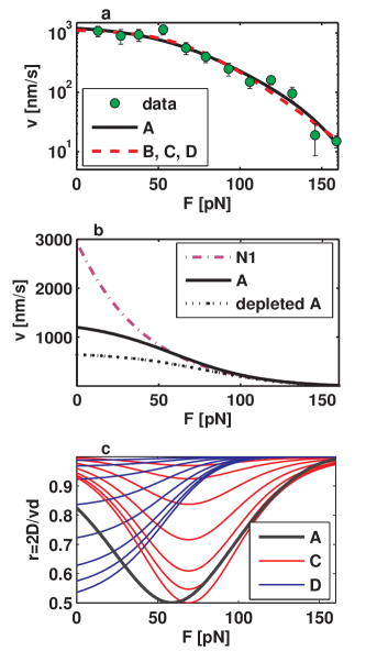
Figure 2: Force velocity relations for pilus retraction, parameterizations as defined in table 1. (a) Experimental retraction data for “wild type” N. gonorrhoeae maier04 , full $N=2$ parameterizations A (same as N2), and restricted $N=2$ parameterizations B, C and D. The experiment is well described by the $N=2$ model, and the result for A and N2 is almost indistinguishable from B, C and D. (b) High load analysis as in Ref. maier04 with an $N=1$ model (N1) compared to the A parameterization. Also a model for an ATP-depleted version of A by setting $u_{0}\to 0.5u_{0}$. The ATP-depleted velocity tends to the non-depleted result (A) at high loads, in qualitative agreement with experimental findings maier02 . Also, the $N=1$ and $N=2$ models agree at high load. (c) Predicted randomness $r=2D/vd$ for the different parameterizations A (and N2), C and D. Parameters B is the limit $R_{C}\to 0$ of C, which is the lowest curve. The lowest curve of the D parameter family is the limit $R_{D}\to 4(u_{0}^{(\mathrm{B})})^{2}/u_{1}^{(\mathrm{B})}\approx 175$ s^-1. The C and D families predict qualitatively different behavior, which should make it possible to distinguish experimentally between them even though they give exactly the same velocity. Also note that $0.5$ is a strict lower bound on randomness for models of this kind with $N=2$ koza02 .

Some parameters in N2 are extremely small, and can be put to zero without any significant difference in velocity, which is how the A parameterizations is constructed. This does not imply that one reaction is completely irreversible, which would violate detailed balance reimann , but rather that one backward rate is small enough to be negligible in the fit.

There is no obvious relation between the load distribution lengths of A and N1, which is surprising since N1 is a good description of the high force regime. It is therefore tempting to ask whether the force velocity relation can be equally well described by other parameterizations, with at least one irreversible step and only one force-dependent step. The minimal way to do this is to remove the backward step completely from A. This constrained parameterization, B, cannot be statistically rejected even at 80% confidence. However, the rate-limiting step in B is still twice as large in N1, a result which is retained even if only high forces are considered (not shown). The reason for this difference is the presence of a force independent step. To show this, we rewrite the $N=1$ velocity in the form of an $N=2$ model with two equal consecutive reactions. For simplicity, we neglect the weak force dependence of the backward rate. With the notation $p^{(\mathrm{X})}$ for parameter $p$ in parameterization $X$, we get:

$$v^{(\mathrm{N1})}=\frac{2d^{(\mathrm{N1})}\Big{(}(u_{0}^{(\mathrm{N1})})^{2}e^{-2d_{0}F^{(\mathrm{N1})}/k_{\mathrm{B}}T}-(w_{0}^{(\mathrm{N1})})^{2}\Big{)}}{2\big{(}u_{0}^{(\mathrm{N1})}e^{-Fd_{0}^{(\mathrm{N1})}/k_{\mathrm{B}}T}+w_{0}^{(\mathrm{N1})}\big{)}}$$ (4)

At forces where the numerator is dominating the force dependence, this is similar to an $N=2$ model with one force independent step and twice as long load distribution length on the other step. The factor 2 in numerator and denominator shows the fact that the elementary step is also twice as long, if the denominator is brought to the same form as Eq. (2), with four terms. We conclude that the plateau in $v(F)$ at low loads have implications for the interpretation of data at high loads, and that the earlier estimate of the elementary step in Ref. maier04 is too small by (at least) a factor 2.

The B parameterization has another interesting property. It has exactly the same force velocity relation as two different parameter families, C and D, which we now describe. To construct C from B, one adds an arbitrary force independent backward reaction. To keep the velocity unchanged, the force dependent forward rate must be modified, but all other parameters in B are kept.

$$\begin{array}[]{l@{\,,\;}l@{\,,\;}l}w_{1}^{(\mathrm{C})}=R_{C}&d_{1}^{(\mathrm{C})}=0&u_{1}^{(\mathrm{C})}=u_{1}^{(\mathrm{B})}\Big{(}\frac{u_{0}^{(\mathrm{B})}+R_{C}}{u_{0}^{(\mathrm{B})}}\Big{)}\end{array}$$ (5)

Here, the constant $R_{C}$ is non-negative but otherwise arbitrary, and we retrieve the B model in the limit $R_{C}\to 0$. To construct the D parameter family from B, we move the load dependence from the forward step to a new (arbitrary) backward rate, and modify both forward rates.

$$\begin{array}[]{lcl}w_{1}^{(\mathrm{D})}=R_{D},&R_{D}>(2u_{0}^{(\mathrm{B})})^{2}/u_{1}^{(\mathrm{B})},&d_{1}^{(\mathrm{D})}=c_{1}^{(\mathrm{B})}\\ \lx@intercol u_{0,1}^{(\mathrm{D})}=\frac{u_{1}^{(\mathrm{B})}R_{D}}{2u_{0}^{(\mathrm{B})}}\bigg{(}1\pm\sqrt{1-\frac{(2u_{0}^{(\mathrm{B})})^{2}}{u_{1}^{(\mathrm{B})}R_{D}}}\;\bigg{)}\hfil\,,\;&c_{1}^{(\mathrm{D})}=0\end{array}$$ (6)

$R_{D}$ again defines a parameter family, and the choice of sign in the lower equation is irrelevant for $v$ and $D$.

$X$	comment	$k_{X}$	-$2\ln L_{\text{X}}$	parameters
N2	full $N=2$ model	8	130.69	$\begin{array}[]{l@{=\,}l}du_{0}&1.35\cdot 10^{3}\\ c_{0}&3.6\cdot 10^{-14}\\ du_{1}&1.24\cdot 10^{4}\\ c_{1}&0.162\\ dw_{0}&2.9\cdot 10^{-14}\\ d_{0}&4.4\cdot 10^{-14}\\ dw_{1}&14.3\cdot 10^{-3}\\ d_{1}&0.311\end{array}$
A	$w_{0}$, $c_{0}=0$	5	130.69	Same as N2 except $w_{0}$, $c_{0}=0$
B	$w_{0}$, $c_{0}$, $w_{1}=0$	3	132.14	$\begin{array}[]{l@{=\,}l}du_{0}&1.15\cdot 10^{3}\\ du_{1}&3.02\cdot 10^{4}\\ c_{1}&0.202\end{array}$
N1	$N$=1 model $F>60$ pN only	4	-	$\begin{array}[]{l@{=\,}l}du_{0}&2.4\cdot 10^{3}\\ c_{0}&0.104\\ dw_{0}&39\\ d_{0}&3.2\cdot 10^{-9}\end{array}$

Table 1: Maximum likelihood estimates of parameters. The products $du_{i}$, $dw_{j}$ are given in units of nm/s, and load lengths are in nm. $d$ is the (unknown) lattice period. $L_{\text{X}}$ is the maximum value of the likelihood function and $k_{X}$ the number of free parameters in parameterization $X$. If $X$ is constructed from parameterization $Y$ by constraining some parameters in $Y$, $X$ is rejected in favor of $Y$ if $2\ln(L_{Y}/L_{X})$ is larger than the upper $\alpha$-percentile of a $\chi^{2}$ distribution with $(k_{Y}-k_{X})$ degrees of freedom, where $1-\alpha$ is the chosen level of confidence NISTstatistics . A cannot be rejected in favor of N2; there is practically no difference. Even at only 80% confidence, B cannot be rejected in favor of N2 or A. An unrestricted fit of the behavior at high load to an $N=1$ model gives the N1 parameters, reproducing the analysis of Ref. maier04 .

Using the obtained parameters, we can compute the diffusion constant $D$. In the context of molecular motors, diffusion is commonly analyzed in terms of the dimensionless randomness parameter $r=2D/vd$ fisher03 ; fisher01 ; svoboda94 ; fisher00 ; koza02 ; chen02 , which is shown in Fig. 2c. The randomness is convenient in this case, as it is independent of $d$, which is unknown for the PilT motor. Although parameterizations B, C and D give equivalent force-velocity relations, they make different predictions for the diffusion constant. We see that B and C make qualitatively different predictions than D, and that A is quite close to B at high forces, but deviating at $F<60$ pN. We expect a measurement of the diffusion constant $D$ would discriminate between the different parameterizations. N2 is again indistinguishable from A (not shown).

The velocity dependence on ATP concentration ([ATP]) has been studied in experiments on ATP depleted bacteria, and two regimes where found maier02 . At low loads, the velocity was strongly dependent on [ATP], but at high loads, the velocity was the same for the depleted strain as for the undepleted strain (“wild type”). A simple way to include ATP dependence in a mechanochemical step model is to make one forward rate (‘binding reaction‘) proportional to [ATP]. Figure 2b shows the velocity relation for the A parameters with the load independent forward rate reduced by 50%. We see that the difference compared to the original A parameters vanishes for high load, in qualitative agreement with the experimental result maier02 . Adding the [ATP] dependence to the other step gives qualitatively different dependence (not shown). Also note that if [ATP] dependence is added to the restricted parameterizations B-D in this way, they still predict the same velocity for all loads and [ATP].

Conclusion

We interpret pilus retraction data on wild type N. gonorrhoeae in terms of a mechanochemical model, which is a discrete random walk with steps between nearest neighbors. Despite its simplicity, a description in these terms contains interesting information about the free energy landscape of the retraction reactions fisher03 ; fisher01 ; bustamante00 .

We find that the experimental data for retraction velocity is well described for all measured forces by several parameterizations, all of which have one effectively force independent step and one irreversible step. The model also captures the qualitative behavior of varying [ATP], namely that the [ATP] dependence of velocity is strong at low force and very weak at high force maier02 . As expected, the binding reaction is not force dependent, but the unbinding might be.

We find several different parameterizations that give similar or identical velocities, but make very different predictions for the diffusion constant $D$ of the retraction. Without any assumptions regarding the elementary step $d$, we predict the randomness $r=2D/dv$ as shown in Fig. 2c, which would be of considerable interest to study experimentally. Such measurements may be able to distinguish the different parameterizations (A, B, C and D) and lead to additional important insight into the pilus retraction mechanism.

We use a model that can account for the all measured forces, we make predictions open to experimental test, and we get new result for the elementary step $d$: $0.5$ nm for parameterization A and $0.2$ nm for the B, C and D parameters, compared to $0.1$ nm for the $N=1$ model maier04 . As we argued above, the short step may be an artifact of using a model with too few states to describe a restricted part of the force-velocity curve. Adding another state to account for the behavior at low loads changes the interpretation of the high load behavior.

Even if we get at least twice as long step as in Ref. maier04 , it is still not obvious how our result fits with the known facts about the system. Each pilin subunit contributes about $0.8$ nm to the filament length maier04 ; maier02 ; mattick ; pilstruct , hence one would like to account for at least one pilin subunit in a complete description of a reaction cycle. In this light, our work is a great improvement even if there are still a few Ångström left to account for. One possibility is that a model with more states could account for the missing length, just like going from one state to two states did. Another is that the strong forces deform the sub-states and destroy the correspondence between load lengths and physical lengths bustamante00 . Since the existing data is well described by our model, this question must probably be settled experimentally. There is also a length associated with the involved energies and forces: at the maximal measured force, $160$ pN, the free energy gain from hydrolysis of one ATP molecule under physiological conditions ($\approx 80$ pN nm boal ; howard ) is enough to retract $0.5$ nm. The evidence that retraction is powered by ATP hydrolysis maier02 does not imply that it is powered only by ATP hydrolysis. The above estimate indicates that more energy than that of one ATP is needed to retract one subunit. Since PilT forms a hexamer, it may hydrolyze up to six ATP in parallel, which would explain the high force energetically. Another possibility is that free energy from depolymerization of the filament is used in retraction. It might be possible to resolve details of for example a second binding event with a model with more states. However, models with more states have more parameters, so more experimental data is needed to explore these exciting possibilities.

This work extends previous physical modeling of the PilT system maier04 in several ways. In particular, the fluctuations (randomness parameter) emerge as a key property for further theoretical and experimental study of the dynamics of pilus retraction.

References

- (1) Mattick, J. S. (2000) Annu. Rev. Microbiol. 56, 289–314.
- (2) Forest, K. T. & Tainer, J. A. (1997) Gene 192, 165–169.
- (3) Merz, A.J., So, M., & Sheetz, M. P. (2002) Nature 407, 98–101.
- (4) Sun, H., Zusman, D. R., & Shi, W. (2000) Curr. Biol. 10, 1143–1146.
- (5) Skerkar, J. M. & Berg, H. C. (2001) Proc. Natl. Acad. Sci. USA 98, 6901–6904.
- (6) Forest, K. T., Satyshur, K. A., Worzalla, G. A., Hansen, J. K., & Herdendorf, T. J. (2004) Acta Crystallogr. D 60, 978–982.
- (7) Maier, B., Koomey, M., & Sheetz, M. P. (2004) Proc. Natl. Acad. Sci. USA 101, 10961–10966.
- (8) Maier, B., Potter, L., So, M., Seifert, H. S., & Sheetz, M. P. (2002) Proc. Natl. Acad. Sci. 99, 16012–16017.
- (9) Boal, D. (2002) Mechanics of the Cell. (Cambridge University Press).
- (10) Howard, J. (2001) Mechanics of Motor Proteins and the Cytoskeleton. (Sinauer Associates Inc.).
- (11) Svoboda, K., Mitra, P., & Block, S. M. (1994) Proc. Natl. Acad. Sci. 91, 11786.
- (12) Fisher, M. E. & Kolomeisky, A. B. (1999) Proc. Natl. Acad. Sci. 96, 6597–6602.
- (13) Kolomeisky, A. B. & Fisher, M. E. (2000) Physica A 279, 1–20.
- (14) Fisher, M. E. & Kolomeisky, A. B. (2001) Proc. Natl. Acad. Sci. 98, 7748–7753.
- (15) Kolomeisky, A. B. & Fisher, M. E. (2003) Biophys. J. 84, 1650.
- (16) Derrida, B. (1983) J. Stat. Phys. 31, 433–450.
- (17) Kolomeisky, A. B. & Widom, B. (1997) J. Stat. Phys. 93, 633–645.
- (18) Keller, D. & Bustamante, C. (2000) Biophys. J. 78, 541–556.
- (19) Reimann, P. (2002) Phys. Rep. 361, 57–265.
- (20) Baker, J. E. (2003) J. Theor. Biol.
- (21) Press, W. H., Vetterling, W. T., Teukolsky, S. A., & Flannery, B. P. (1995) Numerical Recipes in C. (Cambridge University Press).
- (22) (2005) NIST/SEMATECH e-Handbook of Statistical Methods. (NIST).
- (23) Koza, Z. (2002) Phys. Rev. E 65, 031905.
- (24) Chen, Y., Yan, B., & Rubin, R. J. (2002) Biophys. J. 83, 2360–2369.