Quantification of the differences between quenched and annealed averaging for RNA secondary structures

Abstract

The analytical study of disordered system is usually difficult due to the necessity to perform a quenched average over the disorder. Thus, one may resort to the easier annealed ensemble as an approximation to the quenched system. In the study of RNA secondary structures, we explicitly quantify the deviation of this approximation from the quenched ensemble by looking at the correlations between neighboring bases. This quantified deviation then allows us to propose a constrained annealed ensemble which predicts physical quantities much closer to the results of the quenched ensemble without becoming technically intractable.

I Introduction

Heteropolymer folding is of crucial significance in molecular biology. It is the basis for the mechanism with which cells can produce three dimensional building blocks out of the one-dimensional information stored in their genome. Cells achieve this by forming (still one-dimensional) polymers (proteins and RNA) by stringing together different monomers with covalent bonds. All monomers share a compatible backbone but they have different side chains and occur in a predefined order along the sequence. Physical interactions between these monomers force the polymer to stably fold into a three dimensional structure. This structure is crucial for the function of the molecule; it is determined by the specific sequence of the polymer dill95 ; onuch97 ; garel97 ; shakh97 .

In addition to its biological relevance, heteropolymer folding is also a very interesting problem of statistical mechanics higgs00 ; higgs96 ; pagna00 ; hart01 ; pagna01 ; bund02 ; krzak02 ; marin02 ; muller02 ; orland02 ; mukho03 ; baiesi03 ; leoni03 . The competition between the configurational entropy of the polymer, the overall tendency of the monomers to stick to each other, the sequence disorder, and the preference of folding toward a biologically active native state, leads to a very rich thermodynamic phase diagram. While the same qualitative behavior is expected for proteins and RNA, we will here concentrate on RNA since RNA folding is more amenable to analytical and numerical approaches than protein folding. The relative simplicity of the RNA folding problem compared to the protein folding problem does not stem from the fact that RNA consists of only four different bases versus the twenty amino acids the proteins are composed of, but it comes from the simpler interaction rules: The dominant interaction between the four bases A, U, G, and C of an RNA molecule is Watson-Crick (G–C and A–U) pair formation, i.e., if two bases have formed a pair they to first order do not take part in any further interactions. Every amino acid of a protein on the contrary interacts with all its spatial neighbors, i.e., with on the order of ten other amino acids at a time.

From a statistical physics point of view, the possibility of a glass phase at low temperatures driven by sequence disorder, is of special interest in the heteropolymer folding problem higgs96 ; pagna00 ; hart01 ; pagna01 ; bund02 ; krzak02 ; marin02 . Unfortunately, even for the case of RNA folding an analytic quantitative description of the glass phase is still outstanding. Thus, quantitative studies have to either rely on numerics or they have to use what is known as the annealed average. In the annealed average, the free energy of the system is approximated as the logarithm of the ensemble averaged partition function (instead of taking the ensemble average over the logarithm of the partition function called the quenched average). Physically, this approximation corresponds to treating the sequence degrees of freedom as dynamical instead of frozen variables. Thus, the annealed system represents a sequence ensemble that is coupled to the structural ensemble by way of the interaction energies. This sequence ensemble may be different from the original sequence ensemble of uncorrelated random sequences over which the free energy is supposed to be averaged. Due to these differences between the annealed and the quenched sequence ensemble the annealed free energy is only an approximation to the true (quenched) free energy of a disordered system.

The purpose of this manuscript is to first quantify the differences between the annealed and the quenched sequence ensembles. Specifically, we will look at correlation between neighboring bases. We show that while this correlation is strictly zero in the correct (quenched) sequence ensemble, they are non-zero in the annealed sequence ensemble and increase with decreasing temperature - up to complete correlation in certain models of RNA folding. This clearly underlines and quantifies the fundamental shortcomings of the annealed average in the RNA folding problem at low temperatures.

Based on the quantified non-zero nearest neighbor correlations, we then try to diminish the differences between the annealed and quenched ensembles by forcing the annealed ensemble to present zero neighboring correlation. This constrained annealed ensemble behaves much more similar to the quenched ensemble than the annealed ensemble. Although the glass phase itself can not be identified using the constrained annealed ensemble which only partially corrects the overall non-random correlations, one can obtain thermodynamic quantities which are much closer to the quenched results than the annealed ones using this method.

This paper is organized as follows: In Sec. II, we briefly review the RNA secondary structure and introduce the general RNA folding problem with sequence disorder. In Sec. III, we quantify the deviation of nearest neighbor correlations of the annealed ensemble. Finally, we improve the pure annealed ensemble by applying a constraint of random correlations in Sec. IV.

II RNA folding problem with sequence disorder

II.1 RNA secondary structures

RNA is a single-stranded biopolymer of four different bases A, U, C, and G. The strand can fold back onto itself and form helices consisting of stacks of stable Watson-Crick pairs (A with U or G with C). This comparatively simple interaction scheme makes the RNA folding problem very amenable to theoretical approaches without losing the overall flavor of the general biopolymer folding problem higgs00 .

An RNA secondary structure S is characterized by its set of Watson-Crick base pairs $(i,j)$ where $i$ and $j$ denote the $i^{th}$ and $j^{th}$ base of the RNA polymer respectively (conventionally $i<j$). Here, we follow many previous studies higgs00 ; higgs96 ; pagna00 ; hart01 ; pagna01 ; bund02 ; krzak02 ; marin02 ; muller02 ; orland02 ; mukho03 ; baiesi03 ; leoni03 and apply the reasonable approximation to exclude so-called pseudoknots tinoco , i.e., for two Watson-Crick pairs $(i,j)\in{\bf S}$ and $(k,l)\in{\bf S}$, configurations with $i<k<j<l$ are not allowed. This approximation is justified, because short pseudoknots do not contribute much to the overall energy and long pseudoknots are kinetically difficult to form.

II.2 Quenched averaging

The properties of RNA folding, especially the possibility of a glass phase driven by the sequence disorder, have been a challenging problem from the statistical physics points of view. To understand the statistics of this disordered system, one first has to assign an energy $E(\chi,{\bf S})$ to every secondary structure S for a given sequence $\chi$. This could, e.g., simply be the negative of the total number of Watson-Crick base pairs. This then allows us to calculate the partition function

$$Z(\chi)=\sum_{{\bf S}}\cap(\chi,{\bf S})e^{-E(\chi,{\bf S})/T}$$ (1)

for a given sequence $\chi$ where $\cap(\chi,{\bf S})$ is one when the secondary structure ${\bf S}$ is compatible with the sequence $\chi$ and zero otherwise. Finally, one has to calculate the quenched average

$$F_{q}=-k_{B}T\langle\ln Z(\chi)\rangle_{\chi}$$ (2)

over all sequences $\chi$.

II.3 Annealed averaging

Unfortunately, the quenched free energy $F_{q}$ is very difficult to calculate. Thus, one can try to approximate the quenched free energy by the much easier computed annealed free energy, which treats the disordered sequences as dynamic variables. This annealed free energy is only a lower bound of the quenched free energy,

$$F_{a}=-k_{B}T\ln\langle Z(\chi)\rangle_{\chi}<F_{q}.$$ (3)

It can be quite different from the quenched free energy since the annealed ensemble favors those sequences where more binding pairs are allowed. More importantly, physical quantities derived from this annealed free energy can be very different from their quenched counterparts as we will show explicitly in the following sections. To be specific, we will measure the correlation between neighboring bases which are known to vanish in the quenched case.

II.4 Energy models

In this paper, we study the simplest model of disordered RNA sequences which contain only the two bases A and U. In assigning free energies to secondary structures, we neglect any loop entropies and focus on the base pairs alone. Besides, for most parts of this manuscript, we do not consider the minimal hairpin length constraint which requires the two bases of a binding pair to be separated by at least three bases in a real RNA molecule. Within these approximations we do consider two different energy models.

In the binding energy model, we simply assign an energy $\epsilon=-1$ to each AU (or UA) binding pair. We denote the corresponding Boltzmann factor by $q=e^{1/T}$. This model captures the main features of the energetics and is simple enough for analytical and numerical studies.

We also study a somewhat more realistic energy model, namely the stacking energy model. In this model, we assign energies to the stacking of two base pairs rather than to individual base pairs. This stacking energy depends in reality on the identities of all four bases involved. We implement this effect by associating a Boltzmann factor $s_{1}$ with stackings of types ${AA\atop UU}$ and ${UU\atop AA}$ while associating a different Boltzmann factor $s_{2}$ with stackings of types ${AU\atop UA}$ and ${UA\atop AU}$. To be specific, we will choose these Boltzmann factors as $s_{1}=e^{2/T}$ and $s_{2}=e^{1/T}$ for the remainder of this communication.

The main reason to study the stacking energy model is that the simple binding energy model is known to be pathological without a glass phase at low temperature in the disordered sequence ensemble pagna00 ; hart01 ; pagna01 . A simple reason is that whatever the sequence, each base A can always find another base U to pair with provided we have the same amount of bases A and U. Thus, sequences disorder does not cause frustration. In contrast, the energy distribution of the stacking energy model is greatly affected by sequences, and a structure in which all base pairs are stacked can in general not be found for every sequence. Thus, sequence disorder is expected to cause frustration, and a glass phase is expected in this energy model for low enough temperature.

III Nearest neighbor correlations of the annealed ensemble

In this section, we calculate quantitatively how the nearest neighbor correlations in the annealed ensemble deviate from their true values in the random sequence ensemble. To this end, we have to calculate the annealed partition function for sequences with length N-1, which is defined as

$$Z_{a}(N)=\frac{1}{2^{N-1}}\sum_{{\bf S}}\left(\sum_{\chi}\cap(\chi,{\bf S})e^{-E(\chi,{\bf S})/T}\right).$$ (4)

Figure 1: Recursive relation exploring all possible secondary structures for a homogeneous sequence of length N. The wavy lines stands for contribution from all possible structures and sequences. The straight line stands for non-paired bases.

For the binding energy model, this annealed partition function can be easily obtained via the recursive relation shown in Fig. 1 along the lines of previous studies degenn68 ; water78 ; zuker84 ; mccas90 ; bund02 but taking the sequences into account explicitly. The idea is to separate the two cases for the last base, which is either unbound or bound to a certain base k, and then relate the partition function to the shorter length one as

$$Z_{a}(N+1;q) = Z_{a}(N;q)$$

$$+ \frac{q}{2}\sum_{k=1}^{N-1}Z_{a}(k;q)Z_{a}(N-k;q).$$

With this relation, one can obtain an analytical formula for the annealed partition function in the large N limit by performing the z-transform, which is defined as

$$\widehat{Z_{a}}(z;q)=\sum_{N=1}^{\infty}Z_{a}(N;q)z^{-N},$$ (6)

on the recursive relation. After solving the resulting quadratic equation for $\widehat{Z_{a}}(z;q)$, we can obtain the partition function by doing the inverse z-transform,

$$Z_{a}(N;q)=\frac{1}{2\pi i}\oint\widehat{Z_{a}}(z;q)z^{N-1}dz.$$ (7)

This approach can be easily generalized to the stacking energy model.

In order to keep track of the correlations by the annealed ensemble, we assign an additional Boltzmann factor $L$ to all AA and UU neighbors within the sequence. The modified annealed partition function is then

$$Z_{a}(N;q,L)=\frac{1}{2^{N-1}}\sum_{{\bf S}}\left(\sum_{\chi}\cap(\chi,{\bf S})q^{n_{q}({\bf S})}L^{n_{L}({\chi})}\right),$$ (8)

where $n_{q}({\bf S})$ is the number of binding pairs in a secondary structure ${\bf S}$, and $n_{L}({\chi})$ is the number of conjugate neighbors, i.e., AA and UU neighbors in the sequence.

The additional Boltzmann factor complicates the calculation of the partition function since different bases A and U contribute differently. However, we can still formulate recursive relations by noticing that the two end bases of a sequence piece determine the correlations with other pieces. Thus, we can separate a sequence into two cases where the end bases are either of the same type or not, and formulate the recursive relation for each case independently. The annealed partition function $Z_{a}(N;q,L)$ is then obtained via z-transform as before. Since the formation of the recursive relations is quite technical, we only address the result here, and defer the details to Appendix A.

From the partition function we can obtain the nearest neighbor correlations by looking at the deviation of the averaged fraction of AU (or UA) neighbors from the expected value 1/2 in the disordered sequence ensemble. This deviation $\delta$ is obtained by taking the derivative as

$$\delta=\frac{1}{2}-\frac{1}{N}L\partial_{L}\ln(Z_{a}(N;q,L))|_{L=1}.$$ (9)

III.1 Binding energy model

Figure 2: Deviation of the fraction of AU (or UA) nearest neighbors. The deviation is plotted as a function of temperature in units of the binding energy for the binding energy model. Notice that the deviation moves further away from zero and stops at a fixed constant as temperature decreases. It also approaches a limit larger than zero at high temperature indicated by the dashed line.

Fig. 2 shows the neighbor correlations for the binding energy model. We find that the deviation moves further away from zero as temperature decreases. This is a direct result from the fact that at low temperature, the main contributions to the annealed partition function come from those sequences which allow a lot of binding pairs, unlike the quenched case where sequences are equally weighted.

The exact way that the neighbor correlations are biased can be understood as follows. In this binding energy model, the only thing that biases the nearest neighbor correlations is the formation of minimal hairpins since they enforce the neighboring bases to be different, which are either AU or UA. Thus, the degree of bias is directly coupled to the fraction of smallest hairpins in a sequence.

This assertion can be verified by studying the fraction of minimal hairpins. As an example, we study the zero temperature case where all the bases are expected to be paired. Among all possible pairing structures, we explicitly calculate the fraction of smallest hairpins (with the details shown in Appendix B). As a result, every fourth base is part of a minimal size hairpin. Thus, we have $1/4$ AU (or UA) nearest neighbors from these hairpins and another $1/2\times 3/4=3/8$ from the rest of the bases since they do not show nearest neighbor correlation bias. The deviation of the fraction of AU (or UA) neighbors is then expected to be $5/8-1/2=1/8$, which matches exactly the zero temperature limit in Fig. 2. In this case, the sequence, as a dynamic variable, adjusts itself to all the binding pairs.

Even in the high temperature limit, although all allowed sequences are equally weighted, there still exists a finite fraction of minimal size hairpins on average. As a result, the deviation of neighbor correlations approaches a constant larger than zero.

The assertion that the deviation $\delta$ is coupled to the formation of minimal size hairpins is again verified as we additionally require all the hairpins being of length larger than one. In this case, the correlation between nearest neighbors becomes random at all temperatures. However, the second nearest neighbor correlations become non-trivial.

This simple binding energy model gives us a taste how the nearest neighbor correlations are coupled with the energy through the structure, i.e., the formation of minimal hairpins. This correlation is biased since the annealed ensemble puts more weight on lower energy sequences.

III.2 Stacking energy model

Following the same approach, we check the same deviation as a function of temperature in the more realistic stacking energy model. Again, only the result is quoted here in Fig. 3 (interested readers can check the detailed calculations in Appendix C).

Figure 3: Deviation of the fraction of AU (or UA) nearest neighbors for the energy model involving stacking energies. Unlike in the case of the binding energy model, the AU (or UA) neighbor correlations are completely biased at zero temperature in the stacking energy model. At high temperature, this deviation approaches the same limit as the binding energy model.

Unlike the binding energy model, at zero temperature, the nearest neighbor correlations of the stacking energy model are completely biased. Almost no AU (or UA) neighbors can be found in this annealed system. This can be understood since at zero temperature, the only dominating structure is a long stem in which all stacking loops are of type $s_{1}$. Thus, the only two important sequences are the ones made of half consecutive A bases and the other half of U bases.

To verify this structure, we additionally introduce another Boltzmann factor $h$ for each hairpin loop formation. With this Boltzmann factor we can keep track of the fraction of hairpins $f_{h}$ in the annealed system by calculating

$$f_{h}=\frac{1}{N}h\partial_{h}\ln(Z_{a}(N;s_{1},s_{2},h,L=1))|_{h=1}.$$ (10)

From Fig. 4, we do see that the fraction of hairpins of this annealed system indeed goes to zero as temperature goes to zero, which is a feature of the long stem structure.

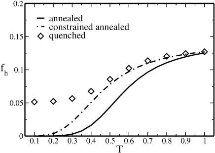
Figure 4: Fraction of hairpins in the stacking energy model for three different ensembles.

At high temperature, however, the energy model does not matter since entropy dominates. Thus, the AU (or UA) fraction approaches the same limit as in the binding energy model.

From this stacking energy model, we learn that the stronger the energy is coupled to the nearest neighbor correlations, the larger deviation in nearest neighbor correlations of the annealed system will be present at low temperature.

IV Constrained annealing

So far we have only observed the sequence correlations artificially introduced through the annealed ensemble. However, our approach can in fact be used to generate more realistic ensembles within the annealed framework. The idea is to force the nearest neighbor correlations to be random when performing the annealed average morita64 ; orlandi02 .

We simply enforce this random disorder constraint, i.e., the fraction of AU (or UA) neighbors being one half by setting the Boltzmann factor $L$, which controls the nearest neighbor correlations, to whatever value it needs to have for the correlations of the annealed ensemble to vanish.

This constrained annealing turns out to predict thermodynamic quantities much closer to the quenched results. And it can be done immediately following our quantified deviations in disorder.

IV.1 Binding energy model

The constraint for the binding energy model is read as

$$\frac{1}{N}L\partial_{L}\ln(Z_{a}(N;q,L))|_{L=L_{c}}=\frac{1}{2}.$$ (11)

In this energy model, we expect the sequences with more AU (or UA) nearest neighbors to be suppressed since the annealed system favors those neighbors. As a result, $L_{c}$, which favors AA (or UU) neighbors, is expected to be larger than one in order to meet the constraint. Furthermore, $L_{c}$ should be larger at lower temperatures since the neighbor correlation is more biased at lower temperatures.

One important note is that the resulting free energy is only defined up to an additive constant, i.e., adding a constant background potential does not change the result at all. Thus, the absolute value of this constrained annealed free energy as well as the Boltzmann factor $L_{c}$ has no real meaning. For example, one could assign the Boltzmann factor $L$ to AU (or UA) neighbors instead of AA (or UU) neighbors. The resulting chemical potential would then change a sign and the free energy would differ by a constant amount. However, the thermodynamic quantities, which are calculated by taking derivatives of the constrained free energy, will not see this constant and are expected to be closer to the quenched result.

To verify this assertion, we are going to compute the average fraction of binding pairs for the binding energy model via $q/N\partial_{q}\ln(Z_{a}(N;q,L))$ as a function of temperature. Then, we compare the cases of the annealed ($L=1$), the constrained annealed ($L=L_{c}$) and the quenched ensembles.

As to the quenched result, we numerically calculate the partition function given random sequences of length 1280 and collect the data from 1000 random sequences. In order to avoid the trivial finite size effects due to fluctuation of the fraction of A bases away from its expected value 1/2, we only choose sequences that contain exactly 640 A’s and 640 U’s. The result is shown in Fig. 5. The statistical errors of the quenched results are always smaller than the size of the corresponding symbol, such that within the error bars the quenched results never overlap other curves. This condition holds for all other quenched results in this manuscript.

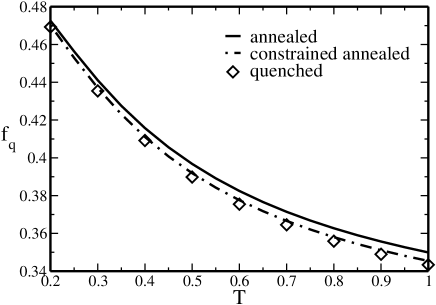
Figure 5: Fraction of binding pairs in the binding energy model. The constraint of random nearest neighbors brings the annealed quantity closer to the quenched numerical estimate. The statistical errors of the quenched results are always smaller than the size of the symbol.

We see that the constrained annealed result is indeed very close to the quenched numerical estimate. However, all three results are rather close to each other anyway. The reason for these three cases being so close to each other is simply that under this energy model the system is not glassy, and every base is able to find another base for pairing in this binding energy model. Thus, at zero temperature, all the bases are paired in all three systems. The fact that the nearest neighbor correlations are not biased a lot can also be verified as we find that at T=0.1, $L_{c}$ to be just 1.59. Thus, the chemical potential introduced from the constraint is comparatively small and does not affect the result too much.

IV.2 stacking energy model

The situation for the stacking energy model is very different from that of the binding energy model. Here, we follow the same approach and compute the averaged fraction of stacking loops of type ${AA\atop UU}$ (or ${UU\atop AA}$) and ${AU\atop AU}$ (or ${UA\atop UA}$) as a function of temperature under the constraint,

$$\frac{1}{N}L\partial_{L}\ln(Z_{a}(N;s_{1},s_{2},h=1,L))|_{L=Lc}=\frac{1}{2}.$$ (12)

Similarly, in order to avoid the trivial finite size effects for the quenched numerical estimate, we fix the number of AA, AU, UA, UU neighbors in the randomly chosen sequences to be 320 each altsch85 .

Figure 6: Fraction of stacking loops ${AA\atop UU}$ (or ${UU\atop AA}$) in the stacking energy model. The constraint of random nearest neighbors fixes this quantity much better than averaged number of pairs in the binding energy model. The phenomenological constraint, i.e., a fixed fraction of hairpins, brings this quantity only a bit closer to the quenched result.

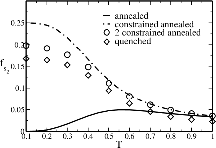
Figure 7: Fraction of stacking loops ${AU\atop UA}$ (or ${UA\atop AU}$) in the stacking energy model. Again, the constraint of random nearest neighbors greatly improves the result. However, unlike the case in Fig. 6, the constraint of a fixed fraction of hairpins also contributes in bringing the annealed quantity closer to the quenched result.

From Figs. 6 and  7, we see that the constrained annealed results are greatly improved over the plain annealed results. This verifies the idea that larger deviations from the random disorder result in a better correction via the constraint of the random disorder. For this stacking energy model, at T=0.1, $L_{c}$=0.0067 is much more different from 1 than in the binding energy model.

From these results, we can see that the constrained annealed ensemble of the stacking energy model behaves in the following way. Since the ensemble is forced to have the same number of AA (or UU) and AU (or UA) neighbors, at zero temperature, the dominating structure is still a long stem structure, but with half the stacking loops being of type $s_{1}$ and the other half being $s_{2}$. This is consistent with the fact that fraction of hairpins going to zero as temperature goes to zero for the constrained annealed system as shown in Fig. 4 .

One difference between the quenched ensemble and the constrained annealed ensemble is that not all the bases of a random sequence can form stacking loops. Thus, we have a finite fraction of hairpins in the quenched ensemble (Fig. 4). This difference can used as an additional phenomenological constraint to improve the constrained annealed system even further.

We apply this additional phenomenological constraint by requiring the fraction of hairpins $f_{h}$ to fit the quenched numerical estimates and neighboring bases to be uncorrelated at the same time, i.e., to enforce

$$\frac{L}{N}\partial_{L}\ln(Z_{a}(N;s_{1},s_{2},h,L))|_{h=h_{c},L=L_{c}}\! \!=\! \!\frac{1}{2}$$ (13)

$$\frac{h}{N}\partial_{h}\ln(Z_{a}(N;s_{1},s_{2},h,L))|_{h=h_{c},L=L_{c}}\! \!=\! \!f_{h}(T),$$ (14)

where $f_{h}(T)$ is the quenched numerical estimate in this equation.

From Figs. 6 and 7, we see that this additional constraint slightly improve the fraction of stacking loops $s_{1}$, but significantly improves the fraction of stacking loops $s_{2}$. This can be understood since the existence of hairpins introduces AU (or UA) neighbors, if the fraction of AU (or UA) neighbors is also required to be one half, it will decrease the fraction of stacking loops $s_{2}$ among the stem structures.

V Conclusion

We conclude that the deviation of the annealed ensemble from the quenched ensemble is strongly related to the energy model and can be completely biased when the correlation is strongly coupled to the energy of the system. Quantifying this deviation allows us to do constrained annealing which brings the predictions of thermodynamic quantities much closer to the real values in the quenched ensemble. As the deviation is larger, the constraint is stronger and thus brings the annealed ensemble even closer to the quenched results. Unfortunately, the biasing toward the quenched ensemble is not strong enough to actually drive the system into the glass transition.

Besides the nearest neighbor correlations, one could also consider the correlations for next nearest neighbors or even two bases separated by arbitrary distances. In principle, all these correlations together would bring us to the exact quenched results and thus to the glass transition. However, the calculations become much more cumbersome as one increases the distance between the two bases, and are left for future work.

VI Appendix

VI.1 Annealed partition function for the binding energy model

The annealed partition function is obtained by first summing over all compatible sequences given a secondary structure S and then summing over all possible structures S, which can be done via the recursive relation in Fig. 1. We define the annealed partition function for a sequence of length N as $Z_{a}(N+1)$. In addition, the annealed partition function for a sequence of length N with its two end bases paired is defined as $A_{e}(N-1)$. The recursive relation in Fig. 1 is then read as

$$Z_{a}(N+1)=\frac{1+L}{2}Z_{a}(N)+\sum_{k=1}^{N-1}\frac{1+L}{4}Z_{a}(k-1)A_{e}(N-k).$$ (15)

The factor $(1+L)/2$ for the first term on the right hand side comes from the contribution in nearest neighbor correlations between the free base N and base N-1, and the 2 takes care of averaging over the number of sequences. We have a similar factor in the second term coming from the correlation between base k of the arch and base k-1. In the later part we will show that the behavior of the annealed partition function is mainly determined by the arch term $A_{e}$, so we will only look at this quantity here. The first base of $A_{e}$ is also specified to be A and the last base to be the conjugate base U.

Figure 8: Recursive relation for the annealed partition function over heterogeneous sequences where the first and the last bases form a conjugate pair. A letter ’E’ is used to denote that the two bases at the ends of the arch are conjugate bases.

Again, the annealed partition function for the arch can be obtained through a similar recursive relation (Fig. 8). The two terms on the right hand side are further decomposed in Figs. 9 and 10.

Figure 9: Decomposition of an arch with its last base inside being a free base, which can be either A or U, into two cases. The letter ’O’ is used to denote that the two bases at the ends of the arch are non-conjugate.

Figure 10: Separation of arches.

In these relations, we need to keep track of two factors: the energy contributions and the nearest neighbor correlations. From the energetic point of view, an arch can be thought of simply contributing a Boltzmann factor $q$ and need not stand for a real binding pair, even though initially it is used to represent a real binding pair. Thus, in Fig. 9, as we try to relate the annealed partition function to its shorter length ones, we assume an effective binding pair between bases 1 and N-1 simply to conserve the energy contribution. In this case, the two bases are not really paired.

In order to keep track of the correct nearest neighbor correlations, we use a letter E on an arch to denote that the two bases at the ends of the arch are conjugate bases. Similarly, a letter O is used to represent two non-conjugate bases at the ends of the arch. Thus, in Fig. 9, the two cases where base N-1 is either A or U are separated and are denoted by letter E and O, which is determined by whether the bases 1 and N-1 are conjugate or not. These notations enable us to connect the decomposed terms recursively back to the relation in Fig. 8.

In Fig. 10, an inner arch can be treated as a free base in considering the energy and correlations for the rest of the bases outside the inner arch. However, there is a difference in counting neighbor correlations for this treatment because the free base looks as a base A from the right, but as a base U from the left. The correct correlations can be obtained if we shift this discrepancy to the last base and flip it from U to A. Thus, the last term carries a letter O on the arch instead of E.

These recursive relations are then read as

$$A_{e}(N-1) = \frac{L}{2}A_{e}(N-2)+\frac{1}{2}A_{o}(N-2)+$$

$$\frac{1}{4}\sum_{k=2}^{N-2}A_{e}(N-k-1)\left[LA_{o}(k-1)+A_{e}(k-1)\right],$$

$$A_{o}(N-1) = \frac{L}{2}A_{o}(N-2)+\frac{1}{2}A_{e}(N-2)+$$

$$\frac{1}{4}\sum_{k=2}^{N-2}A_{e}(N-k-1)\left[LA_{e}(k-1)+A_{o}(k-1)\right].$$

Together with the initial conditions, $A_{e}(1)=q$, $A_{e}(2)=qL$, $A_{o}(1)=qL$, $A_{o}(2)=q(1+L)/2$, one can solve for $A_{e}(N)$ by performing the z-transform

$$\widehat{A_{e}}(z) = \sum_{N=1}^{\infty}A_{e}(N)z^{-N},$$ (18)

$$\widehat{A_{o}}(z) = \sum_{N=1}^{\infty}A_{o}(N)z^{-N},$$ (19)

on the recursive relations. After solving for $\widehat{A_{e}}(z)$, $A_{e}(N)$ can be obtained through the inverse transform

$$A_{e}(N)=\frac{1}{2\pi i}\oint\widehat{A_{e}}(z)z^{N-1}dz.$$ (20)

From previous studies bund02 , we know that in the thermodynamic limit, the partition function has an analytical form as $A_{e}(N)\propto N^{-3/2}z_{c}(q,L)^{N}$, where $z_{c}(q,L)$ is the greatest real part among the branch points obtained from the solution of $\widehat{A_{e}}(z)$.

Similarly, if we perform z-transform on equation 15, we can relate the z-transform of the annealed partition function $\widehat{Z_{a}}(z)$ to that of the arch $\widehat{A_{e}}(z)$. Since these two share the same branch points, the asymptotic behavior of the annealed partition function is different from the above formula for the arch by just a different prefactor, which does not play a role in the thermodynamic limit.

The fraction of AA (or UU) neighboring bases per base of the annealed system is then easily calculated as $L\partial_{L}\ln(z_{c}(q,L))|_{L=1}$. Unfortunately, the analytical solution of this set of polynomial equations is too cumbersome to convey any useful information. Thus, we resort to numerical evaluation of this analytical solution in this paper.

VI.2 Fraction of minimal hairpins at zero temperature

As discussed in the main text, the fraction of minimal size hairpins can be easily obtained once we figure out the partition function. At zero temperature, the partition function is simpler than the finite temperature one since we only need to consider the ground states where all bases are paired. This partition function is obtained through the recursive relation in a similar way as shown in Fig. 11.

Figure 11: Recursive relation for the partition function where all the bases are paired.

We define the partition function for a sequence of length 2(N-1) as $Z_{m}(N,h)$, where $h$ is the Boltzmann factor for a minimal size hairpin. The recursive relation is then read as

$$Z_{m}(N+1)=\sum_{k=1}^{N-1}Z_{m}(k)Z_{m}(N-k+1)+hZ_{m}(N).$$ (21)

Together with the initial conditions, $Z_{m}(1)=1$ and $Z_{m}(2)=h$, one can obtain the asymptotic behavior through z-transform. After simple algebra, we have the largest pole $z_{c}(h)=h+2\sqrt{h}+1$ for the z-transform of partition function $\widehat{Z_{m}}(z,h)$. The partition function $Z_{m}(N)$ is then proportional to $z_{c}(h)^{N}$.

The fraction of minimal size hairpins per two bases is then easily calculated as

$$\partial_{h}\ln z_{c}(h)|_{h=1}=\frac{1+1/\sqrt{h}}{h+2\sqrt{h}+1}|_{h=1}=1/2.$$ (22)

Thus, the fraction of minimal size hairpins per base is 1/4.

VI.3 Annealed partition function for the stacking energy model

The calculation for the stacking energy model follows the same approache. However, it is a bit more complicated since we need to keep track of stacking loops involving four bases which leads us to the recursive relation depicted in Fig. 12.

Figure 12: Recursive relation for the stacking energy model.

In these recursive relations, we use an additional letter S on the arch to denote the fact that we consider the stacking energy of the stacking loop formed partly by that binding pair. Independent of the type of the arch, all the stacking energies inside the arches are still considered in all cases. Thus, the first term on the right hand side in Fig. 12 does not contain an S because its base N-1 is unbound, and no stacking loop can be formed with the binding pair of the arch.

Figure 13: Decomposition of the annealed partition function which last base inside the arch is a free base.

Similar to the recursive relation in previous section, we then discard the last base as a free base as shown in Fig. 13. Again, the arches on the right hand side are meant to preserve the energy contributions only. In the second line of the relation, we further decompose the terms in order to relate these terms with the first recursive relation in Fig. 12.

Figure 14: Separation of arches considering the hairpin contribution.

In Fig. 14, we also separate the contributions of the inner arch from the rest part as in Fig. 10. One difference is that we consider the contribution from the hairpin loops in this case. Thus, the hairpin loop contained in the outer arch term is not a real hairpin loop because of the existence of the inner arch. The correct result is obtained by adding the last term in the relation.

In this stacking energy model, we denote the annealed partition function for an arch of length N-1 as $A_{es}(N)$. The recursive relations are then read as follows

$$A_{es}(N\!-\!1)\! = \!\frac{L}{2}\left(A_{es}(N\!-\!2)\!-\!(s_{1}\!-\!1)\frac{(1+L^{2})}{4}A_{es}(N\!-\!4)\right)+\frac{1}{2}\left(A_{os}(N\!-\!2)\!-\!(s_{2}\!-\!1)\frac{2L}{4}A_{es}(N\!-\!4)\right)+\frac{s_{1}L^{2}+s_{2}}{4}A_{es}(N\!-\!3)$$

$$+ \!\frac{1}{4}\sum_{k=3}^{N\!-\!2}A_{es}(N\!-\!k\!-\!1)\left[L\left(A_{os}(k\!-\!1)\!-\!(s_{1}\!-\!1)\frac{2L}{4}A_{es}(k\!-\!3)\right)+\left(A_{es}(k\!-\!1)\!-\!(s_{2}\!-\!1)\frac{1+L^{2}}{4}A_{es}(k\!-\!3)\right)+2(\frac{1}{h}\!-\!1)H_{o}(k)\right],$$

$$A_{os}(N\!-\!1)\! = \!\frac{L}{2}\left(A_{os}(N\!-\!2)\!-\!(s_{1}\!-\!1)\frac{2L}{4}A_{es}(N\!-\!4)\right)+\frac{1}{2}\left(A_{es}(N\!-\!2)\!-\!(s_{2}\!-\!1)\frac{1+L^{2}}{4}A_{es}(N\!-\!4)\right)+\frac{s_{1}L+s_{2}L}{4}A_{es}(N\!-\!3)$$

$$+ \!\frac{1}{4}\sum_{k=3}^{N\!-\!2}A_{es}(N\!-\!k\!-\!1)\left[L\left(A_{es}(k\!-\!1)\!-\!(s_{1}\!-\!1)\frac{1+L^{2}}{4}A_{es}(k\!-\!3)\right)+\left(A_{os}(k\!-\!1)\!-\!(s_{2}\!-\!1)\frac{2L}{4}A_{es}(k\!-\!3)\right)+2(\frac{1}{h}\!-\!1)H_{e}(k)\right],$$

where the terms $H_{e}$ and $H_{o}$ stand for the contribution from a hairpin. They are obtained separately from a recursive relation similar to the one in Fig. 9, by just replacing the wavy line by a straight line, which means that bases are not bound. One can then easily formulate the recursive relations for $H_{e}$ and $H_{o}$.

Together with the initial conditions: $A_{es}(1)=h$, $A_{es}(2)=hL$, $A_{es}(3)=h(1+3L^{2}+s_{2}+s_{1}L^{2})/4$, $A_{os}(1)=hL$, $A_{os}(2)=h(1+L^{2})/2$, $A_{os}(3)=h(3L+L^{3}+s_{1}L+s_{2}L)/4$, we can perform z-transform to obtain the asymptotic behavior of the annealed partition function for the stacking energy model.

References

- (1) K. A. Dill et al., Protein Sci. 4, 561 (1995).
- (2) J. N. Onuchic, Z. Luthey-Schulten, and P. G. Wolynes, Annu. Rev. Phys. Chem. 48, 545 (1997).
- (3) T. Garel, H. Orland and E. Pitard, J. Phys. I (France) 7, 1201 (1997).
- (4) E. I. Shakhnovich, Curr. Opin. Struct. Biol. 7, 29 (1997).
- (5) P. G. Higgs, Q. Rev. BioPhys. 33, 199 (2000).
- (6) P. G. Higgs, Phys. Rev. Lett. 76, 704 (1996).
- (7) A. Pagnani, G. Parisi and F. Ricci-Tersenghi, Phys. Rev. Lett. 84, 2026 (2000).
- (8) A. K. Hartmann, Phys. Rev. Lett. 86, 1382 (2001).
- (9) A. Pagnani, G. Parisi and F. Ricci-Tersenghi, Phys. Rev. Lett. 86, 1383 (2001).
- (10) R. Bundschuh and T. Hwa, Phys. Rev. E 65, 031903 (2002).
- (11) F. Krzakala, M. Mézard and M. Müller, EuroPhys. Lett. 57, 752 (2002)
- (12) E. Marinari, A. Pagnani and F. Ricci-Tersenghi, Phys. Rev. E. 65, 041919 (2002)
- (13) M. Müller, F. Krzakala and M. Mézard Euro. Phys. J. E. 9, 67 (2002).
- (14) H. Orland, and A. Zee, Nucl. Phys. B. 620, 456 (2002)
- (15) R. Mukhopadhyay, E. Emberly, C. Tang and N. S. Wingreen, Phys. Rev. E. 68, 041904 (2003)
- (16) M. Baiesi, E. Orlandini and A. L. Stella, Phys. Rev. Lett. 91, 198102 (2003)
- (17) P. Leoni and C. Vanderzande, Phys. Rev. E. 68, 051904 (2003)
- (18) I. Tinoco Jr. and C. Bustamante, J. Mol. Biol. 293, 271 (1999), and references therein.
- (19) P. G. de Gennes, Biopolymers 6, 175 (1968).
- (20) M. S. Waterman, Advances in Mathematics, Supplementary studies, edited by G.-C. Rota (Academic, New York, 1978), pp.167-212.
- (21) J. S. McCaskill, Biopolymers 29, 1105 (1990)
- (22) M. Zuker and D. Sankoff, Bull. Math. Biol. 46, 591 (1984)
- (23) T. Morita, J. Math. Phys. 5, 1401 (1964)
- (24) E. Orlandini, A. Rechnitzer and S. G. Whittington, J. Phys. A. 35, 7729 (2002)
- (25) S. F. Altschul and B. W. Erickson, Mol. Biol. Evol. 2, 526 (1985)