The Transition from Anti-Parallel to Component Magnetic Reconnection

Abstract

We study the transition between anti-parallel and component collisionless magnetic reconnection with 2D particle-in-cell simulations. The primary finding is that a guide field $\approx\thinspace\negthickspace 0.1$ times as strong as the asymptotic reconnecting field — roughly the field strength at which the electron Larmor radius is comparable to the width of the electron current layer — is sufficient to magnetize the electrons in the vicinity of the x-line, thus causing significant changes to the structure of the electron dissipation region. This implies that great care should be exercised before concluding that magnetospheric reconnection is antiparallel. We also find that even for such weak guide fields strong inward-flowing electron beams form in the vicinity of the magnetic separatrices and Buneman-unstable distribution functions arise at the x-line itself. As in the calculations of Hesse et al. [2002] and Yin and Winske [2003], the non-gyrotropic elements of the electron pressure tensor play the dominant role in decoupling the electrons from the magnetic field at the x-line, regardless of the magnitude of the guide field and the associated strong variations in the pressure tensor’s spatial structure. Despite these changes, and consistent with previous work, the reconnection rate does not vary appreciably with the strength of the guide field as it changes between $0$ and a value equal to the asymptotic reversed field.

SWISDAK ET AL. TRANSITION GUIDE FIELD M. Swisdak, Icarus Research, Inc., PO Box 30780 Bethesda MD 20824-0780, USA , (swisdak@ppd.nrl.navy.mil)

1 Introduction

The fast dissipation of magnetic energy in collisionless plasmas is a common occurrence in nature, with examples ranging from tokamak sawtooth crashes to magnetospheric substorms to solar flares. The process common to these phenomena is thought to be magnetic reconnection, in which oppositely directed components of the magnetic field cross-link, forming an x-line configuration. The expansion of the newly connected field lines away from the x-line converts magnetic energy into kinetic energy and heat while pulling in new flux to sustain the process.

Observations suggest that in many systems the ratio of the characteristic reconnection time to the Alfvén crossing time is $\sim 0.1$. The simplest magnetohydrodynamic (MHD) description of reconnection [Sweet, 1958; Parker, 1957] is inconsistent with this value, being too slow by several orders of magnitude [Biskamp, 1986]. However, the numerical simulations comprising the GEM Reconnection Challenge [Birn et al., 2001] showed that the inclusion of the Hall effects, which are important at small spatial scales and are neglected in MHD, can produce fast reconnection. The magnetic topology in these simulations was understandably quite simple: equal and anti-parallel fields separated by a thin current layer. Yet even in the magnetotail, where this approximation is often close to reality, a small field directed parallel to the current (a guide field) is often observed [Israelovich et al., 2001].

The effects of a guide field, $B_{g}$, on magnetic reconnection have been examined before. Sharp differences have been seen in the large-scale flows around the x-line [Hoshino and Nishida 1983; Tanaka 1995; Pritchett 2001] as well as the pressure and magnetic field signatures [Kleva et al., 1995; Rogers et al. 2003]. Three-dimensional particle simulations of similar systems without [Zeiler et al. 2002] and with [Drake et al., 2003] a guide field showed that the former was basically laminar in the direction parallel to the guide field while the latter developed strong turbulence. Pritchett and Coroniti [2004] noted that moderate guide fields ($B_{g}/B_{0}\lesssim 1$, where $B_{0}$ is the reconnecting field) have only a slight effect on the reconnection rate, although Ricci et al. [2004] found somewhat slower rates for larger fields ($B_{g}/B_{0}=3,5$). Hesse et al. [1999,2002] and Yin and Winske [2003] showed that non-gyrotropic electron motions balance the reconnection electric field at the x-line in both the anti-parallel and guide field cases.

In light of these results, determining the minimum guide field $B_{g}$ that changes the structure of the x-line becomes of interest. If it satisfies $B_{g}>B_{0}$ then the effects of a guide field can usually be ignored in the magnetosphere. On the other hand, if the transition occurs when $B_{g}<<B_{0}$ guide-field reconnection is typical, and anti-parallel is a special case perhaps only relevant in simulations. We argue, based on both simulations and theoretical grounds, that the transition occurs when the electron Larmor radius in the guide field at the x-line becomes smaller than the width of the electron current layer, ${\it i.e.}$ for $B_{g}/B_{0}\approx 0.1$. The implication is that most magnetospheric reconnection is probably component reconnection.

In section 2 of this paper we present our computational scheme and initial conditions. Section 3 presents results for the case $B_{g}=0$, section 4 for $B_{g}=1.0$ and section 5 for $B_{g}=0.2$. We summarize our results and discuss their implications for understanding magnetospheric reconnection in section 6.

2 Computational Details

Our simulations are done with p3d, a massively parallel particle-in-cell code [Zeiler et al., 2002] . The electromagnetic fields are defined on gridpoints and advanced in time with an explicit trapezoidal-leapfrog method using second-order spatial derivatives. The Lorentz equation of motion for each particle is evolved by a Boris algorithm where the velocity $\mathbf{v}$ is accelerated by $\mathbf{E}$ for half a timestep, rotated by $\mathbf{B}$, and accelerated by $\mathbf{E}$ for the final half timestep. To ensure that $\bm{\nabla\cdot}\mathbf{E}=4\pi\rho$ a correction electric field is calculated by inverting Poisson’s equation with a multigrid algorithm.

The equations solved by the code are written in normalized units. Masses are normalized to the ion mass $m_{i}$, the magnetic field to the asymptotic value of the reversed field, and the density to the approximate value at the center of the current sheet (see below). Other normalizations derive from these: velocities to the Alfvén speed $v_{A}$, lengths to the ion inertial length $c/\omega_{pi}=d_{i}$, times to the inverse ion cyclotron frequency $\Omega_{ci}^{-1}$, and temperatures to $m_{i}v_{A}^{2}$.

Our coordinate system is chosen so that the inflow and outflow for an x-line are parallel to $\mathbf{\hat{y}}$ and $\mathbf{\hat{x}}$, respectively. The guide magnetic field and reconnection electric field are parallel to $\mathbf{\hat{z}}$. For comparison, our $\mathbf{\hat{x}}$, $\mathbf{\hat{y}}$, and $\mathbf{\hat{z}}$ unit vectors correspond to $-\mathbf{\hat{x}}$, $\mathbf{\hat{z}}$, and $\mathbf{\hat{y}}$ in GSM coordinates. The simulations presented here are two-dimensional in the sense that out-of-plane derivatives are assumed to vanish, i.e., $\partial/\partial z=0$.

The initial equilibrium comprises two Harris current sheets [Harris 1962] superimposed on a ambient population of uniform density. The reconnection magnetic field is $B_{x}=\tanh[(y-L_{y}/4)/w_{0}]-\tanh[(y-3L_{y}/4)/w_{0}]-1$, where $w_{0}=0.25$ and $L_{y}=6.4$ are the half-width of the initial current sheets and the box size in the $\mathbf{\hat{y}}$ direction respectively. This configuration has two current sheets and allows us to use fully periodic boundary conditions. The electron and ion temperatures, $T_{e}=0.05$ and $T_{i}=0.5$, are initially uniform as is the guide field $B_{g}$. Except for the background (lobe) population, which can have arbitrary density (here $n_{\ell}=0.2$), pressure balance uniquely determines the initial density profile. In this equilibrium the density at the center of each sheet is $\approx 1.1$ at $t=0$. At $t=0$ we perturb the magnetic field ($\tilde{B_{x}}/B_{0}\approx 0.1$) to seed x-lines at $(x,y)=(L_{x}/4,3L_{y}/4)$ and $(3L_{x}/4,L_{y}/4)$.

To conserve computational resources, yet assure a sufficient separation of spatial and temporal scales, we take the electron mass to be $0.01$ and the speed of light to be $20$. The domain measures $6.4$ on a side and the grid has $1024\times 1024$ points, which implies that there are $\approx\negmedspace 16$ gridpoints per electron inertial length and $2$ per electron Debye length. To check for convergence we doubled the box size for one run (for $B_{g}=0.2$) and saw no significant variation in our results.

The particle timestep is $6\times 10^{-4}$, or $0.12\omega_{pe}$. Our simulations follow $\sim 10^{9}$ particles and conserve energy to better than $1$ part in $1000$.

3 Overview, $B_{g}=0$

Investigating the critical value of $B_{g}$ with multiple 3-D simulations would entail a prohibitive computational expense, so we instead performed a series of 2-D simulations that varied only in the strength of the guide field. The restricted dimensionality means that many turbulent modes, including the Buneman instability seen by Drake et al. [2003], are not present. However, other investigators have found that the gross morphological features of reconnection x-lines are roughly invariant in the direction parallel to the current density [Pritchett and Coroniti, 2004].

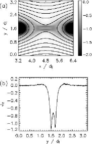
Figure 1: Reconnection in a system with $B_{g}=0$ at $t=4.5$. (a) The out-of-plane current density overlaid with magnetic field lines in a region surrounding the x-line. The blackest regions are not color-coded correctly, having been over-exposed to show details near the x-line (b) A vertical cut through the x-line at $x=4.8$.

A snapshot of the out-of-plane current density near the x-line for a simulation with $B_{g}=0$ is shown in Figure 1. The initial current sheet has completely reconnected; the plasma at the x-line at the time shown was in the low density ($n_{\ell}=0.2$) lobe at the simulation’s beginning. Since $|\mathbf{B}|=0$ at the x-line for $B_{g}=0$ inward-flowing electrons must at some point find themselves in a region where the magnetic field is too weak to dominate their motion. This happens at a distance from the x-line given roughly by the electron inertial length, $c/\omega_{pe}\equiv d_{e}$, which for this simulation is $\sqrt{m_{e}/n_{\ell}}\approx 0.2$ (in normalized units). Once the electrons demagnetize they stream towards the x-line parallel to the $\mathbf{\hat{y}}$ axis, through the region of low magnetic field, until they turn due to the increasing field on the opposite side of the current layer and reverse direction. They then execute “figure-8” trajectories [Speiser 1965], oscillating in the $\mathbf{\hat{y}}$ direction until escaping from the ends of the layer. At the turning points of their trajectories (where $v_{y}\rightarrow 0$), the local electron density increases, forming a bifurcated current sheet. Zeiler et al. [2002] have previously reported this bifurcation, although it is particularly noticeable in our simulations because of the high spatial resolution (16 gridpoints per $d_{e}$) and large ion to electron temperature ratio ($T_{i}/T_{e}=10$). The bifurcation would be obscured in simulations where these parameters had smaller values. Note that this bifurcation is at a much smaller scale than the ion-scale splits reported in Cluster observations [Runov et al. 2003].

The bifurcation is also evident in Figure 2, which shows the diagonal components of the electron temperature. In analogy with the definition of the fluid pressure tensor we define the electron temperature tensor in a grid cell as a sum over the $N$ local particles:

$$T_{\alpha\beta}=\frac{m_{e}}{N}\sum_{i=1}^{N}(v_{\alpha,i}-<\negmedspace v_{\alpha}\negmedspace>)(v_{\beta,i}-<\negmedspace v_{\beta}\negmedspace>)\mbox{,}$$ (1)

where $<\negmedspace\ldots\negmedspace>$ denotes an average, $\it{e.g.,}<\negmedspace x\negmedspace>=\frac{1}{N}\sum_{i=1}^{N}x_{i}$. Like the pressure tensor, which is related to the temperature tensor by $P_{\alpha\beta}=nT_{\alpha\beta}$ where $n$ is the density, the temperature is symmetric, $T_{\alpha\beta}=T_{\beta\alpha}$. For an isotropic plasma the off-diagonal elements of the temperature tensor vanish while the diagonal elements are equal to each other and to the scalar temperature, $T_{\alpha\alpha}=T_{e}$. This is the case at $t=0$ in our simulations.

The decrease in $T_{yy}$ and $T_{zz}$ during inflow are consistent with the adiabatic invariance of the magnetic moment $\mu$: $B\approx B_{x}$ decreases, while $\mu\propto v_{\perp}^{2}/B$ remains constant. $T_{xx}$, approximately the parallel temperature, simultaneously increases due to energy conservation. Any energy change due to the interaction of the reconnection electric field $E_{z}$ and the curvature and grad-$B$ drifts is small everywhere except near the x-line.

Once inside the layer the electrons demagnetize and, as previously seen by Zeiler et al. [2002], the electron distribution in $v_{y}$ space separates into two counter-propagating beams due to the cross-current layer bounce motion (see Figure 2d). As a consequence $T_{yy}$ sharply increases, as has previously been noted by Horiuchi and Sato [1997].

Despite the beams we see no evidence of a two-stream instability, probably because of the small current layer width. Unstable wavenumbers for the electron-two-stream instability satisfy $k_{y}v_{0}<2\omega_{pe}$ where $v_{0}$ is the separation of the beam velocities [Krall and Trivelpiece 1986]. The maximum growth rate, $\gamma=\omega_{pe}/\sqrt{8}$, occurs for $k_{y}v_{0}=\sqrt{3/2}\>\omega_{pe}$, and as $v_{0}\rightarrow 0$ the growth rate vanishes. In the simulation the beam separation is largest at the x-line, $v_{0}\approx 8$, and drops to $0$ at the edges of the layer $\approx 0.22(=d_{e})$ upstream. With a local $\omega_{pe}\approx 90$ the instability criterion implies that only wavelengths $\lambda\gtrsim 0.28$ are unstable at the x-line, and thus that the two-stream instability is not excited in the narrow current layer.

In a 2-D collisionless plasma the reconnection electric field at the x-line is ultimately balanced by the divergence of the electron pressure tensor [Vasyliunas 1975]. In our units the collisionless electron fluid momentum equation is

$$\mathbf{E}=-\mathbf{v_{e}}\mathbf{\times B}-\frac{1}{n_{e}}\mathbf{\nabla\cdot}\mathbf{\bar{\bar{P}}_{e}}-m_{e}(\mathbf{v_{e}\cdot}\mathbf{\nabla})\mathbf{v_{e}}-m_{e}\frac{\partial\mathbf{v_{e}}}{\partial t}$$ (2)

which is exact insofar as the pressure tensor $\mathbf{\bar{\bar{P}}_{e}}$ incorporates all kinetic effects not included in the other terms. The reconnection electric field is thus

$$\begin{split}E_{z}&=-(v_{x}B_{y}-v_{y}B_{x})\\ &-\frac{1}{n}\left(\frac{\partial P_{xz}}{\partial x}+\frac{\partial P_{yz}}{\partial y}\right)\\ &-m\left(v_{x}\frac{\partial{v_{z}}}{\partial x}+v_{y}\frac{\partial{v_{z}}}{\partial y}+\frac{\partial v_{z}}{\partial t}\right)\end{split}$$ (3)

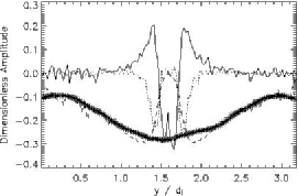
Figure 3: For $B_{g}=0$ a cut through the x-line at x = $4.8$ showing the various terms balancing $E_{z}$ in equation (3). $E_{z}$ is shown by the stars and the dashed, solid, and dotted lines denote the $\mathbf{v\times B}$, divergence of the pressure tensor, and inertial terms, respectively. To reduce the noise the plotted quantities were averaged over 20 gridpoints in x and 4 in y.

where we have dropped the electron subscript and used the fact that $\partial/\partial z=0$. In a steady state only the pressure terms can balance $E_{z}$ at the x-line, as can be seen in Figure 3. Far from the current layer the EMHD relation $\mathbf{E}=-\mathbf{v_{e}\times B}$ holds, while nearer the x-line both the off-diagonal elements of the pressure tensor and the inertial terms are important. At the x-line the pressure tensor terms dominate. Both $\partial P_{yz}/\partial y$ and $\partial P_{xz}/\partial x$ contribute, although the former is larger in our simulation by a factor of $\approx 2$. The term proportional to $\partial/\partial t$ is not shown separately but, as expected during quasi-steady reconnection, is negligible.

4 Guide Field, $B_{g}=1.0$

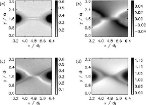
Figure 4: The electron density and out-of-plane magnetic field $B_{z}$ in simulations with $B_{g}=0$ and $1.0$. (a) $n_{e}$, $B_{g}=0$; (b) $B_{z}$, $B_{g}=0$; (c) $n_{e}$, $B_{g}=1.0$; (d) $B_{z}$, $B_{g}=1.0$. In all panels $t=4.5$. In panels (a) and (c) black areas have been over-exposed to show detail at the x-line.

A large guide field changes the structure of the x-line by both lowering the total plasma $\beta$ and magnetizing the electrons throughout the current sheet. When $B_{g}$ is small the dominant wave mode at small lengthscales, and hence the governor of the particle dynamics, is the whistler. This is seen when electrons in the outflow region are accelerated by $E_{z}$ and drag the magnetic field out of the reconnection plane [Mandt et al., 1994; Shay et al., 1998], causing the well-known quadrupolar symmetry in $B_{z}$ along the separatrices [Sonnerup, 1979; Terasawa, 1983] . As $B_{g}$ increases the importance of the kinetic Alfvén mode grows [Rogers et al., 2001]. For that mode the coupling occurs when $E_{||}$ accelerates electrons along newly reconnected field lines, increasing the electron density on one side of the current layer, decreasing it on the other, and forming a quadrupolar pattern [Kleva et al., 1995]. The perturbations in $B_{z}$ acquire a component determined by pressure balance, leading to a symmetric component that can, for very large $B_{g}$, overwhelm the quadrupolar pattern [Rogers et al., 2003]. Figure 4 shows the electron density and $B_{z}$ from the simulation discussed in the previous section ($B_{g}=0$) and one that is otherwise identical except that $B_{g}=1.0$.

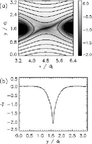
Figure 5: Reconnection in a system with $B_{g}=1.0$ at $t=4.5$. (a) The out-of-plane current density overlaid with magnetic field lines in a region surrounding the x-line. Black areas have been over-exposed to show detail at the x-line. (b) A vertical cut through the x-line at $x=4.8$.

The parallel velocity of the electrons, mostly directed out of the reconnection plane, develops a quadrupolar symmetry opposite to that of the density (high density paired with low velocity and vice versa). The density asymmetry is a larger effect, however, and the result is an out-of-plane current density that is canted with respect to the initial current sheet, as can be seen in Fig. 5. Because inflowing electrons remain magnetized in the guide field they do not have figure-8 trajectories at the x-line and the bifurcations in the electron density and current density disappear.

In the $B_{g}=0$ simulation discussed in Section 3 the magnetic field on the inflow axis ($x=4.8$) was dominantly parallel to $\mathbf{\hat{x}}$ (except at the x-line where $|\mathbf{B}|=0$). For $B_{g}=1.0$, in contrast, the field rotates $\approx 45^{\circ}$ between the lobe plasma and the x-line. The rotation complicates the interpretation of the temperature tensor of equation (1), so to simplify we transform to a coordinate system where the axes are parallel and perpendicular to the local magnetic field. In this frame

$$\mathbf{\bar{\bar{T}}}=[T_{||}\mathbf{\hat{b}\hat{b}}+T_{\perp}(\mathbf{\bar{\bar{I}}}-\mathbf{\hat{b}\hat{b}})]+\mathbf{\bar{\bar{T}}_{ng}}$$ (4)

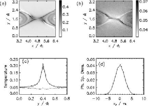
Figure 6: Data for $B_{g}=1.0$. Panels (a) and (b) show $T_{||}$ and $T_{\perp}$, respectively. Panel (c) shows vertical cuts at $x=4.8$. The solid line is $T_{||}$ and the dashed $T_{\perp}$. Panel (d) shows the distribution of $v_{ey}$ in a region measuring $1.0\medspace d_{e}$ long and $0.5\medspace d_{e}$ high and centered on the x-line.

where $\mathbf{\hat{b}}$ is a unit vector in the direction of the magnetic field, $\mathbf{\bar{\bar{I}}}$ is the unit tensor, and $\mathbf{\bar{\bar{T}}_{ng}}$ contains the non-gyrotropic terms. Images of the parallel and perpendicular temperatures along with cuts through the x-line are shown for $B_{g}=1.0$ in Figure 6a-c.

Conservation of magnetic moment again explains the decrease in $T_{\perp}$ along the inflow direction. Since $B_{g}$ is constant the decrease in $B$ is smaller than was the case in section 3, and the relative decrease of $T_{\perp}$ in Figure 6c is smaller than in Figure 2d. Because the electrons remain magnetized at the x-line, $T_{\perp}$ remains small, in sharp contrast to the results shown in Figure 2. The increase in $T_{||}$ inside the current sheet is due to the intermixing of colder inflowing electrons and electrons accelerated by the parallel electric field along the separatrices. The unimodal distribution function of Figure 6d confirms that the electrons do not execute Speiser-like orbits.

The terms balancing the reconnection field in equation (3) are shown for this case in Figure 7. At the x-line the off-diagonal elements of the pressure tensor again make the primary contribution although, as a comparison of Figures 7 and 3 makes clear, the scale length over which they are important is much smaller than when $B_{g}=0$. This is consistent with the results of Hesse et al. [2002]. Unlike the anti-parallel case the $\partial P_{xz}/\partial x$ term makes the dominant contribution while the $\partial P_{yz}/\partial y$ term is negligible.

5 Transition

For what $B_{g}$ does the transition between the reconnection of Section 3 and that of Section 4 occur? Far from the x-line, where both species are completely magnetized, the guide field cannot play an important dynamical role unless $B_{g}\gtrsim B_{0}$. As a particle approaches the current layer, however, the reconnecting component decreases and the influence of the guide field rises. Qualitatively, $B_{g}$ is important when the associated electron Larmor radius is equal to the spatial scale associated with the x-line.

Consider a system with $B_{g}=0$ and examine the z component of the electron equation of motion under quasi-steady conditions,

$$m_{e}v_{ey}\frac{\partial v_{ez}}{\partial y}=-eE_{z}-\frac{e}{c}(v_{ex}B_{y}-v_{ey}B_{x})-\frac{1}{n}\frac{\partial P_{yz}}{\partial y}\mbox{,}$$ (5)

where we have assumed that derivatives with respect to $x$ can be neglected when compared to those with respect to $y$. In a 2D steady-state system Faraday’s Law implies that $E_{z}$ is relatively uniform (see Figures 3 and 7). Far from the x-line electrons are frozen to the magnetic field and the $E_{z}$ and $\mathbf{v\times B}$ terms are roughly equal. Within the current layer the convective part of the inertial term and the pressure tensor become important, with the transition occurring at some lengthscale $\Delta_{y}$ where the terms balance. If, for simplicity, we restrict our attention to the vertical axis through the x-line, symmetry implies that $B_{y}$ is zero and

$$v_{ez}=\Delta_{y}\Omega_{x,\text{up}}$$ (6)

where $\Omega_{x,\text{up}}=eB_{x,\text{up}}/m_{e}c$ is the cyclotron frequency based on the reconnecting field at $y=\pm\Delta_{y}$. In general $B_{x,\text{up}}$ will be less than the asymptotic reconnecting field. Within this inner scale the electrons carry most of the current, so we also have

$$\frac{4\pi}{c}J_{z}=\frac{4\pi}{c}nv_{ez}\approx\nabla\times\mathbf{B}\approx\frac{\partial B_{x}}{\partial y}$$ (7)

where we have ignored both the displacement current and the contribution from the current due to $\partial B_{y}/\partial x$. Converting derivatives with respect to $y$ to division by $\Delta_{y}$ and combining equations (6) and (7) we find that

$$\Delta_{y}=\frac{c}{\omega_{pe}}=d_{e}$$ (8)

The electron velocity producing the current is $v_{ez}\sim d_{e}\Omega_{x,\text{up}}$.

Now consider the addition of a small ambient guide field. The magnetic field no longer vanishes at the x-line and the electron Larmor radius there is

$$\rho_{g}=\frac{v_{ey}}{\Omega_{e,g}}$$ (9)

where we have taken $v_{ex}\approx 0$ based on symmetry considerations, $\Omega_{e,g}=eB_{g}/m_{e}c$ is the electron cyclotron frequency based on $B_{g}$, and $v_{ey}$ is the electron inflow velocity into the unmagnetized region around the x-line. The guide field will be important when this Larmor radius is smaller than the width of the current layer, $\rho_{g}<\Delta_{y}$.

The major contributors to the electron inflow velocity $v_{ey}$ are the thermal speed and the $\mathbf{E}\times\mathbf{B}$ drift. A Sweet-Parker-like scaling suggests that the ratio of the $\mathbf{E}\times\mathbf{B}$ inflow speed to the outflow speed is equal to the normalized reconnection electric field $E_{z}$. For a wide range of conditions it has been shown [Shay et al., 1999; Shay et al., 2001] that the outflow is roughly equal to the electron Alfvén speed $v_{Ae}$ and $E_{z}\approx 0.1$. In the low-temperature limit ($v_{th}<<v_{E\times B}$) this argument implies that $v_{ey}\approx 0.1v_{Ae}$ and the bound for a dynamically important $B_{g}$ is given by

$$\rho_{g}=\frac{v_{ey}}{\Omega_{e,g}}=\frac{0.1v_{Ae}}{\Omega_{e,g}}<\Delta_{y}=d_{e}$$ (10)

or

$$B_{g}>E_{z}\sim 0.1.$$ (11)

In our simulations $E_{z}$, and hence the transitional value of $B_{g}$, is $\approx 0.2$.

Equation (11) is not valid when the electron thermal speed $v_{the}$ dominates the contribution from the $\mathbf{E}\times\mathbf{B}$ drift. In the high-temperature limit one must substitute $v_{th}$ rather than $v_{E\times B}$ for $v_{ey}$ in equation (9), and the relevant criterion becomes $\beta_{g}<1$ where $\beta$ is evaluated with the lobe density and temperature. In the simulations presented here $v_{the}\approx v_{E\times B}$ and so the critical value of the guide field remains $B_{g}\approx 0.2$.

We note that the estimate for the electron inflow velocity $v_{ye}\approx 0.1c_{Ae}$ is smaller than the counter-streaming velocity of the electrons shown in Fig. 2(d). This is because a local electrostatic field $E_{y}$ develops inside the electron current layer that accelerates the electrons towards the magnetic null. However, this field decelerates the electrons once they cross the null so this electric field does not change the effective electron Larmor radius of the electrons in the guide field.

We have explored the transition from anti-parallel to finite guide field reconnection through a series of simulations with $B_{g}=0$, $0.1$, $0.2$, $0.4$, and $0.75$ and found, in agreement with our above arguments, that simulations with $B_{g}=0.2$ most clearly display characteristics intermediate between $B_{g}=0$ and $B_{g}=1$.

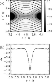
Figure 8: Reconnection in a system with $B_{g}=0.2$ at $t=4.5$. (a) The out-of-plane current density overlaid with magnetic field lines in a region surrounding the x-line. Black areas have been over-exposed to show detail at the x-line. (b) A vertical cut through the x-line at $x=4.8$.

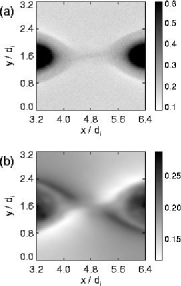
Figure 9: The electron density (a) and out-of-plane magnetic field $B_{z}$ (b) in a simulation with $B_{g}=0.2$. In panel (a) black areas have been over-exposed to show detail at the x-line.

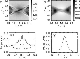
Figure 10: Data from $B_{g}=0.2$. Panels (a) and (b) show $T_{||}$ and $T_{\perp}$, respectively. Panel (c) shows vertical cuts at $x=4.8$. The solid line is $T_{||}$ and the dashed $T_{\perp}$. Panel (d) shows the distribution of $v_{ey}$ in a region measuring $1.0\medspace d_{e}$ long and $0.5\medspace d_{e}$ high and centered on the x-line.

Figure 8 shows the out-of-plane current density for a run identical to those previously discussed except that $B_{g}=0.2$. There is no bifurcation in the current density and the canting of the current layer, while present, is not as strong as the case with $B_{g}=1.0$ (Figure 5). Figure 9 shows the electron density and $B_{z}$ for this simulation. The electron density is not bifurcated and bears some resemblance to the quadrupolar cavities so prominent in Figure 4c, while $B_{z}$, although still basically quadrupolar, no longer has the strong symmetry obvious of Figure 4b. Evidence for a transition can also be seen in the parallel and perpendicular temperatures shown in Figure 10. The results are clearly intermediate between Figures 2 and 6. The cut in Figure 10c shows that the increase in the parallel temperature as electrons approach the x-line is similar in both magnitude and profile to the $B_{g}=0$ case. Within the current layer, however, $T_{||}$ increases to a sharp peak similar to that for $B_{g}=1$. The perpendicular temperature decreases towards the x-line and then, within the layer, rises to a peak. This peak is midway in magnitude between the $B_{g}=0$ and $B_{g}=1$ cases.

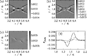
Figure 11: Panels (a)–(c) show the non-gyrotropic component of $P_{yz}$ for $B_{g}=0,0.2,$ and $1.0$. Panel (d) shows a cut at $x=4.8$ in each figure. The solid, dashed, and dotted lines are for, respectively, $B_{g}=0,0.2,$ and $1.0$.

In order to examine the variation with guide field of the off-diagonal pressure tensor terms of Equation 3 it is necessary to separate the gyrotropic and non-gyrotropic contributions. The gyrotropic part is strongly influenced by the presence of a guide field and, in any case, does not contribute to balancing $E_{z}$ at the x-line. Figure 11 shows the change in the non-gyrotropic portion of $P_{yz}$ as the guide field varies. The cuts in Figure 11d demonstrate that as $B_{g}$ increases the role of $\partial P_{yz}/\partial y$ in balancing the reconnection electric field at the x-line decreases dramatically.

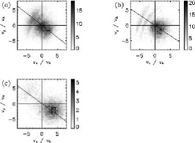
Figure 12: Panels (a)–(c) show the $v_{x}$-$v_{y}$ distribution functions taken just upstream of the separatrix for runs with $B_{g}=0,0.2,1.0$, respectively. The slanted line in each panel shows the direction of the local magnetic field. The colors are measured in units of phase space density. The counter-propagating features at the upper left of each figure are due to electrons accelerated at the x-line

The presence of a small guide field also has signatures far from the x-line. Figure 12 shows the $v_{x}$-$v_{y}$ distribution functions for three simulations with different guide fields taken at the same point, just upstream of the upper-left separatrix and, for the runs with a finite guide field, inside the density cavity. Because of the low plasma density within the cavity the parallel electric field remains finite over an extended region along the separatrix [Pritchett and Coroniti, 2004]) in the $B_{g}=1.0$ system. This electric field locally accelerates the electrons, producing a strong beam flowing towards the x-line. However even for $B_{g}=0.2$ the beam is already clearly present. (The features in the upper left quadrant of each panel are electrons that have already been accelerated at the x-line). There is a net current but no distinct beam for $B_{g}=0$. The origin, detailed structure, and effect of this extended region of $E_{||}$ is discussed in a future publication.

6 Discussion

This study suggests that only a minimal guide field, $B_{g}\approx 0.1B_{0}$ is required to alter the dynamics of electrons both in the vicinity of the x-line and at remote locations along the separatrices. The implication is that in most real systems, including the magnetotail, the guide field might not be negligible. In any case this study suggests that one can not simply ignore the guide field if $B_{g}\ll B_{0}$.

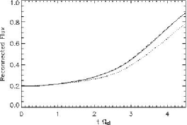
Figure 13: The reconnected flux versus time for the three runs discussed in this work. The solid, dashed, and dotted lines correspond to $B_{g}=0$, $0.2$, and $1.0$, respectively. The reconnection rate is the slope of the curves.

A counter-argument could be made that reconnection with $B_{g}\neq 0$ is significantly slower compared to the case with $B_{g}=0$ and therefore the magnetosphere will self-select locations where the guide field is nearly zero (less than $0.1$ of the anti-parallel field). We find that this is not the case. The guide field alters the dynamics both locally and at large scales significantly before the rate of reconnection is significantly affected. Specifically, Figure 13 shows that magnetic flux reconnects only slightly ($\approx 10$%) slower for $B_{g}=1.0$ than for $B_{g}=0$, a result consistent with other simulations [Rogers et al., 2003; Pritchett and Coroniti, 2004]. It should be noted, however, the the onset of reconnection in real systems could be biased either for or against guide fields. Our simulations do not address this question since they start with a finite perturbation that effectively places the system in the nonlinear regime at $t=0$.

Another factor potentially affecting guide field reconnection is the effect of an ambient pressure gradient and the associated diamagnetic drifts. At the magnetopause, where density gradients perpendicular to the current layer produce diamagnetic drifts, the reconnection rate can be strongly reduced [Swisdak et al., 2003]. However, it was shown that diamagnetic suppression occurs for small guide fields with the transition occurring when $\beta_{x}>B_{g}/B_{0}$ (for density length scales of order an ion inertial length). Combined with the results of this work the conclusion is again that magnetopause reconnection always includes a dynamically important guide field.

Guide fields also play an important role in the development of turbulence in three-dimensional reconnection simulations. Simulations by Drake et al. [2003] with $B_{g}=5.0$ showed that turbulence can self-consistently develop at a reconnection x-line. The acceleration of electrons by the reconnection electric field led to a separation of the ion and electron drift speeds, which then triggered the Buneman instability. At late time the nonlinear evolution led to the formation of electron holes, localized bipolar regions of electric field. These structures produced an effective drag between the ions and electrons that was large enough to compete with the off-diagonal pressure tensor in balancing the reconnection electric field. Earlier 3D simulations with $B_{g}=0$ by Zeiler at al. [2002] produced no significant turbulence at the x-line once reconnection was established. The strong electron heating for $B_{g}=0$ (as shown in Figure 2) suppressed all streaming instabilities near the x-line since for $T_{i}\gg T_{e}$ such instabilities require a beam velocity $v_{b}$ greater than the electron thermal speed $v_{te}$. Yet since $B_{g}=5.0$ is significantly larger than typical magnetospheric values it was unclear from these studies whether turbulence and enhanced ion-electron drag were common features of reconnection in the magnetosphere.

Our 2D simulations cannot produce the Buneman instability at the x-line seen in these earlier simulations. However, we can examine the distribution functions produced by our simulations and determine whether they would be unstable in a full 3D system. In the low temperature limit with $\mathbf{k}$ parallel to both $\mathbf{B}$ and the relative drift velocity $\mathbf{v_{b}}$ a plasma is Buneman unstable to wavenumbers satisfying the relation $kv_{b}<\omega_{pe}$ [Krall and Trivelpiece, 1986]. For finite temperature plasmas with Maxwellian distributions the condition for instability is more complicated and, in fact, for small drifts in warm plasmas no instability exists. The instability threshold for arbitrary distributions can be found numerically, but a rough rule of thumb is that a plasma is Buneman unstable if the electron and ion velocity distribution functions do not substantially overlap ($v_{b}\gtrsim v_{te}$).

Figure 14 shows the distribution of $v_{z}$ at the x-line for runs with three values of the guide field, $B_{g}=0,0.2,1$. The dotted line shows the ion distribution and the double peak is a remnant of the two initial populations, the non-drifting background and the drifting population comprising the initial current sheet. The three electron distribution functions demonstrate that as the guide field increases the x-line electrons acquire a larger drift with respect to the ions. The electron energy gain is limited by the amount of time they spend within the current layer before advecting into the outflow region. Larger simulations suggest that our small system size may prevent the electrons from reaching their maximum speeds. A finite $B_{g}$ acts like a guide wire, restraining this flow and leaving more time for a particle to be accelerated by the reconnection electric field. If our simulation were three-dimensional the $B_{g}=1$ case would almost certainly be Buneman unstable, while the $B_{g}=0$ case would not. Again, the $B_{g}=0.2$ case is transitional.

The small size of the transition guide field has important implications for magnetospheric reconnection. The x-line current sheet should usually be canted with respect to the ambient current layer. Density and flow velocities measured on the separatrices should have a quadrupolar symmetry. Distribution functions taken just upstream of the separatrices should exhibit an inward-flowing beam. Turbulence, and electron holes in particular, should be common. Magnetospheric reconnection with negligible guide fields should be rare.

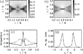
Figure 2: Data for $B_{g}=0$. Panels (a) and (b) show the electron temperatures $T_{xx}$ and $T_{yy}$ (see the text for definitions) near the x-line of Figure 1. Panel (c) shows cuts of the temperatures at $x=4.8$. The solid line is $T_{yy}$, the dashed $T_{xx}$, and the dotted $T_{zz}$. Panel (d) shows the distribution of $v_{ey}$ in a region measuring $1.0\medspace d_{e}$ long and $0.5\medspace d_{e}$ high and centered on the x-line.

Figure 7: The terms balancing the reconnection electric field for $B_{g}=1.0$. $E_{z}$ is shown by the stars and the dashed, solid, and dotted lines denote the $\mathbf{v\times B}$, divergence of the pressure tensor, and inertial terms, respectively. Note the difference in horizontal scale between this figure and Figure 3. To reduce noise the plotted quantities were averaged over 16 gridpoints in x and 4 in y.

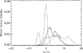
Figure 14: The $v_{z}$ distribution functions for three runs. The solid line shows the case $B_{g}=0$, the dash-dotted $B_{g}=0.2$ and the dashed $B_{g}=1.0$. The dotted line shows the ions.