Modeling spatiotemporal noise covariance
for MEG/EEG source analysis

Abstract

We propose a new model for approximating spatiotemporal noise covariance for use in MEG/EEG source analysis. Our model is an extension of an existing model [1, 2] that uses a single Kronecker product of a pair of matrices - temporal and spatial covariance; we employ a series of Kronecker products in order to construct a better approximation of the full covariance. In contrast to the single-pair model that assumes the same temporal structure for all spatial components, the proposed model allows for distinct, independent time courses at each spatial component. This model better describes spatially and temporally correlated background activity. At the same time, inversion of the model is fast which makes it useful in the inverse analysis. We have explored two versions of the model. One is based on orthogonal spatial components of the background. The other, more general model, is based on independent spatial components. Performance of the new and previous models is compared in inverse solutions to a large number of single dipole problems with simulated time courses and background from authentic MEG data.

1 Introduction

The objective of magnetoencephalography (MEG)/ electroencephalography (EEG) source localization is to infer active brain regions from measurements outside of the human head. Often, for example in evoked response experiments, the data from individual stimulus trials are averaged, time-locked to the stimulus presentation. This averaged post-stimulus signal is compared with the statistical properties of background noise (averaged signal far from the stimulus time) and this difference is used to infer the location and time-courses of neural activity that is, at least on average, generated in response to the given stimulus. Because such inferences are based on differences between signal and background, it is important to characterize the statistical properties of the background as accurately as possible.

The Central Limit Theorem lends support to the common assumption that the averaged background data is Gaussian distributed, even though the distribution of single trial background may not be Gaussian. The log likelihood function is a common mathematical expression quantifying the likelihood that a given model (e.g. of neural current) could have produced the measured data. For Gaussian, zero-mean averaged background noise, the log likelihood function is given by:

$$-\frac{1}{2}\sum_{ktk^{\prime}t^{\prime}}\left[b_{kt}-\int{\mathcal{L}}_{k}(x)j(x,t)dx\right]\mathbf{COV}^{-1}_{kt;k^{\prime}t^{\prime}}\left[b_{k^{\prime}t^{\prime}}-\int{\mathcal{L}}_{k^{\prime}}(x^{\prime})j(x^{\prime},t^{\prime})dx^{\prime}\right].$$ (1)

Here $b_{kt}$ are the averaged measurements (the data being analyzed) at sensor $k$ and time $t$; $j(x,t)$ is the neural (source) current distribution over space $x$ and time $t$; ${\mathcal{L}}_{k}(x)$ is the forward or lead field for sensor $k$ – the linear operator which connects source currents to predicted measurements in the absence of noise. $\mathbf{COV}$ is the covariance of the averaged background activity, which describes second order statistical properties of the MEG/EEG data in the absence of sources. There are a number of different inverse algorithms in use e.g. [3, 4, 5, 6, 7, 8] but most use the likelihood formulation in some way. In all cases, accurate covariance is required to solve the source localization problem reliably. The covariance is commonly taken to be diagonal, even though there is ample evidence that the background is correlated over space and time [9, 10, 11]. This may adversely affect the results of inverse calculations, for example by biasing the locations of reconstructed sources [12].

The sample covariance of the averaged background data is related to the sample covariance of the single-trial background data by a simple expression: $\mathbf{COV}=\frac{1}{M}\widehat{\mathbf{COV}}$. Here, $M$ is the number of trials being averaged and $\widehat{\mathbf{COV}}$ is the sample covariance of the single-trial background data. This relation assumes the trials are independent draws from the single-trial distribution but does not assume a particular form for this distribution. The task of estimating the average background covariance may be accomplished by estimating the single-trial background covariance and scaling it by the number of trials in the average.

Given that MEG/EEG is measured in $M$ trials, on $L$ sensors and in $C$ time samples, let ${\bf E}_{m}$ be the $L\times C$ single trial noise matrix at trial $m$. In this case, the conventional way to estimate the full covariance matrix of dimension $N=LC$ for the averaged noise is by

$$\mathbf{COV} = \frac{1}{M(M-1)}\sum_{m=1}^{M}(vec(\mathbf{E}_{m})-vec(\bar{\mathbf{E}}))(vec(\mathbf{E}_{m})-vec(\bar{\mathbf{E}}))^{T},$$ (2)

$$\bar{\mathbf{E}} = \frac{1}{M}\sum_{m=1}^{M}\mathbf{E}_{m},$$ (3)

where $vec(\mathbf{E})$ is all the columns of $\mathbf{E}$ stacked in a vector. In order to simplify notation in this paper we use symbol $M$ both for the number of available noise samples and for the number of stimuli over which averaging is done. Note that in the general case these numbers may not be the same.

There are a number of reasons why this estimate of the full covariance is difficult to use and why an approximation is needed. First, for modern multi-sensor detectors sufficient experimental data is rarely available to adequately estimate the large number of parameters present in the full covariance matrix. For example, for 35 time samples and 121 channels and considering the fact that the covariance matrix is symmetric, $8,969,730$ parameters should be determined ($(121*35)((121*35)+1)/2$). This far exceeds the amount of data typically available. Second, because the spatiotemporal noise covariance matrix is so large, a tremendous amount of memory is required for its storage. Third, this full covariance is almost impossible to handle in the likelihood formulation, since the computation time of calculating the inverse still renders the task infeasible in most interesting cases, even if it was possible to estimate the covariance with the given data. A naive algorithm for matrix inversion takes $O(N^{3})$ time where $N$ is the dimensionality of the matrix. Though there are some improvements over this result for large matrices [13, 14], the problem is overwhelming for typical computing equipment and for interesting values of $N$. To summarize: it is almost aways impossible to estimate the full spatiotemporal covariance due to lack of data; in those cases when the estimation is possible, the inversion is computationally hard; and in any case the amount of storage required is high. Due to all these difficulties with the estimation of the full spatiotemporal covariance, an accurate approximation is needed. In addition to addressing the above three problems mentioned above a good approximation should capture as much of the structure in the noise as possible and reduce the errors in inverse solutions.

In this paper we describe three different models of increasing complexity and different ways to estimate them (Section 2). The first is the widely used diagonal approximation, which has no spatial or temporal correlation and whose diagonal elements consist of sensor noise variances (Section 2.1). The second model is a Kronecker product approximation of a temporal covariance and a spatial covariance under the assumption that a temporal covariance and a spatial covariance are independent and separable [1]. Parameterized [1] and unparameterized [2] variations of this approximation are available. This paper deals only with the unparameterized approximation estimated in the maximum likelihood framework suggested in [2] (Section 2.2). Two novel and more complex models that do not employ the assumption of independence and separability of temporal and spatial covariance are proposed in Section 2.3 and Section 2.4. The first model is a multi-pair Kronecker product approximation based on orthogonal spatial basis and the second one is a variant based on independent spatial basis.

Since the goal of better noise characterization by covariance modelling is to improve results of inverse algorithms, we have chosen to test and compare all models described in this paper by using them in algorithms for source localization. Performance of the approximations in reconstructing dipole locations and time courses is tested using a large number of simulated single dipole data sets constructed from empirical data for background noise and simulated dipole sources covering a wide range of locations and orientations (Section 3).

2 Models and Methods

This section describes all covariance models compared in this paper. Among them, two novel and relatively more complex models are introduced and explained. Models are presented in the order of increasing complexity.

2.1 Diagonal approximation

It is common when solving the inverse problem to model covariance as a diagonal or even as an identity matrix. In the diagonal case the approximated full spatiotemporal covariance is expressed as $\mathbf{COV}\propto\mathbf{T}\otimes\mathbf{S}$, where T is the temporal covariance which is taken to be the identity; S is the diagonal spatial covariance with elements of the diagonal being sensor variances; and $\otimes$ is the Kronecker product. This model is easy to estimate. It has only $L$ parameters, where $L$ is the number of sensors. At the same time this simple model is better than not using any covariance estimate at all as in the Ordinary Least Squares (OLS) approach.

2.2 Unparameterized Kronecker product model

De Munck et al. [2] proposed a more complex model, based on the assumption that temporal and spatial covariance of the background in MEG and EEG are independent and separable. This allows one to cast spatiotemporal covariance in the form that uses the Kronecker product:

$$\mathbf{COV}\approx\mathbf{T}\otimes\mathbf{S}=\left[\begin{array}[]{cccc}\mathbf{t}_{11}\mathbf{S}&\mathbf{t}_{12}\mathbf{S}&\cdots&\mathbf{t}_{1C}\mathbf{S}\\ \mathbf{t}_{21}\mathbf{S}&\mathbf{t}_{22}\mathbf{S}&\cdots&\mathbf{t}_{2C}\mathbf{S}\\ \vdots&\vdots&&\vdots\\ \mathbf{t}_{C1}\mathbf{S}&\mathbf{t}_{C2}\mathbf{S}&\cdots&\mathbf{t}_{CC}\mathbf{S}\end{array}\right].$$ (8)

Temporal covariance is a $C\times C$ matrix T and spatial covariance is an $L\times L$ matrix S, where $C$ is the number of time samples and $L$ is the number of sensors. In [2] the temporal covariance matrix T is normalized to one. Both matrices are unparameterized. Note, that a single set of variances needs to be divided between the spatial and temporal matrices and that normalization of T takes away a degree of freedom. In this case the number of parameters that need to be estimated equals $L(L+1)/2+C(C-1)/2$. This is less than all elements of both matrices because both are symmetric. These parameters are estimated from the data using a Maximum Likelihood (ML) method as described in [2]. In deriving these ML estimators, the single trial background data was assumed to be Gaussian with a covariance that factored into separate spatial and temporal matrices. This Gaussian distribution was used to construct the likelihood of the single trial background data, from which estimators were derived for the parameters of the spatial and temporal covariance matrices that maximized this likelihood. The resulting estimators are a coupled set of equations between spatial and temporal parameters that may be solved using an iterative technique.

2.3 Orthogonal basis multi-pair model

In the Kronecker product model above, all spatial components of the background have the same temporal covariance structure. This statement describes the main assumption of the single-pair Kronecker product model. In order to motivate multi-pair models, we re-write the single-pair Kronecker product model in the following way. First, perform a spectral decomposition of the spatial covariance:

$$\mathbf{T}\otimes\sum_{l=1}^{L}\sigma^{l}\bm{{\mathcal{S}}}^{l},$$ (9)

where $\bm{{\mathcal{S}}}^{l}=v_{l}v_{l}^{T}$ is an orthonormal basis component represented as a singular matrix. This form is one of the conventional ways of writing a spectral representation of a matrix. Using the identity $\mathbf{A}\otimes(\mathbf{B}+\mathbf{C})=\mathbf{A}\otimes\mathbf{B}+\mathbf{A}\otimes\mathbf{C}$, the expression (9) can be represented as:

$$\sum_{l=1}^{L}\mathbf{T}\otimes\sigma^{l}\bm{{\mathcal{S}}}^{l}=\sum_{l=1}^{L}\sigma^{l}\mathbf{T}\otimes\bm{{\mathcal{S}}}^{l}$$ (10)

The left hand side of the equation (10) makes it obvious that each spatial component has the same temporal covariance. The contribution of each temporal covariance is weighted by the variance of the corresponding orthonormal spatial component, as seen from the right hand side of (10). In the final sum such weighting of temporal covariances makes no difference since they all are the same.

In a more realistic case it is easy to picture a situation where several noise generators having distinct spatial patterns (or, similarly, belonging to separate spatial components) also have different and independent temporal structures. They can have a focal or a distributed spatial pattern that can be described by the corresponding spatial component. Furthermore, some background sources of noise that are external to the head origin can also be captured by such a model.

We propose an alternative multi-pair model of the spatiotemporal noise covariance as a series of orthonormal spatial components $\bm{{\mathcal{S}}}^{l}$ of the background data and their corresponding temporal covariance matrices $\bm{{\mathcal{T}}}^{l}$ expressed as:

$$\mathbf{COV}\approx\sum_{l=1}^{L}\bm{{\mathcal{T}}}^{l}\otimes\bm{{\mathcal{S}}}^{l}.$$ (11)

The model is build on the following assumptions:

1. Spatiotemporal noise is generated by $L$ spatially orthogonal generators which do not change their location during the period of interest.

2. Each spatial component has a time course independent from those of other components.

3. Superposition of time courses of each component measured at the sensors has a Gaussian distribution with zero mean.

Let’s assume for now that we are given the orthonormal components $\bm{{\mathcal{S}}}^{l}$. (We will discuss a way to obtain those later in the section.) As in (9) the orthonormal basis spans the whole sensors space having dimension $L$. The next task is to estimate temporal covariances $\bm{{\mathcal{T}}}^{l}$ of each component. This can be done due to the assumption A3 that the background is Gaussian and using the Maximal Likelihood estimation as demonstrated in the Appendix A. Assume that we have $M$ single trial noise samples $\mathbf{E}_{m}$ – a $L\times C$ matrix with $L$ number of sensors and $C$ number of time points. Now we can summarize orthogonal basis multi-pair model in the following way:

$$\mathbf{COV}\approx\widetilde{\mathbf{COV}} \equiv \sum_{l=1}^{L}\bm{{\mathcal{T}}}^{l}\otimes\bm{{\mathcal{S}}}^{l},$$

$$\bm{{\mathcal{T}}}^{l} = \frac{1}{M^{2}}\sum_{m=1}^{M}\mathbf{E}_{m}^{T}\bm{{\mathcal{S}}}^{l}\mathbf{E}_{m},$$

$$\bm{{\mathcal{S}}}^{l} = v_{l}v^{T}_{l}.$$ (12)

Expression (12) represents a model for the averaged noise hence the normalizing factor in the estimate of $\bm{{\mathcal{T}}}^{l}$ is squared. Note that although the form of expression (11) may suggest that it is a summation of $L$ single pair models, this is not so. Components $\bm{\mathcal{S}}^{l}$ are not covariances and furthermore they are singular because they represent a dimension in an $L$ dimensional space.

Another important feature expected of a covariance model to make it useful in the analysis is a computationally manageable inverse. The inversion of this multi-pair model can be expressed by (see Appendix B for details)

$$\widetilde{\mathbf{COV}}^{-1} = \sum_{l=1}^{L}(\bm{{\mathcal{T}}}^{l})^{-1}\otimes\bm{{\mathcal{S}}}^{l}.$$ (13)

This inversion is easily manageable. Its running time is $O(LC^{3})$, similar to that for the one-pair models.

While this model has far fewer free parameters than the full spatiotemporal covariance estimate (2) the number of parameters is larger than that of models described above (though not by a great amount). The $L$ spatial components $\bm{{\mathcal{S}}}^{l}$ consist of $L(L-1)/2$ parameters plus $LC(C+1)/2$ parameters for all temporal covariances. The increase in parameters provides an increase of expressive power that is greater than of the single pair model (8). Furthermore, it is free from assumptions of identical character of the noise over all spatial locations and hence may capture more information about structure of the noise.

We derived this model without any assumptions about how spatial orthogonal components were obtained. That means that in principle any set of such components should keep the validity of the derivation and retain the invertibility of the model. However, since we assume that the background has the distribution close to the Gaussian then it is natural to use singular value decomposition (SVD) to obtain orthogonal spatial components. In this work we use SVD to estimate the spatial orthogonal components for the orthogonal basis multi-pair model. SVD of the noise data collected in a matrix $\mathbf{A}$ by stacking $M$ single trial spatiotemporal samples $\mathbf{E}_{m}$ looks like $\mathbf{A}=\mathbf{U}\mathbf{\Sigma}\mathbf{V}^{T}$. $\mathbf{U}$ is a $CM\times L$ orthogonal matrix; $\mathbf{\Sigma}$ is an $L\times L$ diagonal matrix with singular values of $\mathbf{A}$ $\lambda_{l}$ as diagonal elements; and $\mathbf{V}$ is an $L\times L$ orthogonal matrix of spatial components. Each row of $\mathbf{V}^{T}$ is a spatial component $v_{l}$ that is used to form orthogonal spatial components $\bm{{\mathcal{S}}}^{l}$ of our model (11).

Very often SVD is used for dimensionality reduction when only the most significant singular values are accounted for and all other values are neglected [15]. In this application we do not use SVD for this purpose. Dimensionality reduction, i.e. approximation of the full covariance is already performed in (11) based on the stated assumptions. The sole purpose of SVD in estimation of this model is finding spatial orthogonal components and their corresponding time courses.

2.4 Independent basis multi-pair model

The model introduced in the previous section has greater expressive power than the models presented previously. Nevertheless, its requirement of orthogonality may be inappropriate for MEG/EEG data. In the general case noise sources do not have to be spatially orthogonal to one another. In an effort to remove this restriction we suggest a generalization, that does not restrict spatial components to be orthogonal. Instead we consider independent spatial components.

Let us assume that we are given independent spatial components of the background. Denote each independent component as $w_{l}$, its corresponding spatial matrix as $\bm{{\mathcal{R}}}^{l}=w_{l}w^{T}_{l}$ and the matrix, in which the $l^{th}$ row is the $w_{l}$ vector, as $\mathbf{W}^{-1}$. In this framework the only assumption needed is independence of each $w_{l}$ from the rest of the components. Estimation of temporal covariances of each independent spatial component can be performed in the Maximum Likelihood framework (see Appendix A).

$$\mathbf{COV}\approx\widetilde{\mathbf{COV}} \equiv \sum_{l=1}^{L}\bm{{\mathcal{T}}}^{l}\otimes\bm{{\mathcal{R}}}^{l}$$

$$\bm{{\mathcal{T}}}^{l} = \frac{1}{M^{2}}\sum_{m=1}^{M}\mathbf{E}_{m}^{T}\mathbf{W}\mathbf{W}^{T}\bm{{\mathcal{R}}}^{l}\mathbf{W}\mathbf{W}^{T}\mathbf{E}_{m}$$

$$\bm{{\mathcal{R}}}^{l} = w_{l}w^{T}_{l}.$$ (14)

Here $w_{l}$ stands for the $l$-th row vector of $\mathbf{W}^{-1}$ as described above and $M^{2}$ is due to the averaged noise modeling.

The model is more general compared to the one using orthogonal bases from Section 2.3. It can be constructed in terms of any spatially independent basis set, which also includes orthogonal sets. The number of free parameters of the model has increased to $L^{2}+LC(C-1)/2$. At the same time its inversion is still manageable and can be expressed as (see Appendix B for details)

$$\widetilde{\mathbf{COV}}^{-1}=\sum_{l=1}^{L}(\bm{{\mathcal{T}}}^{l})^{-1}\otimes[\mathbf{W}\mathbf{W}^{T}\bm{{\mathcal{R}}}^{l}\mathbf{W}\mathbf{W}^{T}].$$ (15)

This makes the model useful in the analysis. However, the computational cost of this operation is greater than that for the orthogonal basis multi-pair model. It is now $O(L(C^{3}+2L^{3})+L^{3})$, where the $2L^{3}$ part comes from repeated multiplication of independent components $\bm{{\mathcal{R}}}^{l}$ by the combination $\mathbf{W}\mathbf{W}^{T}$. The additional $L^{3}$ component is the time to calculate this combination. Nevertheless in localization algorithms, like in the one we used in this study, the covariance matrix does not change across iterations and its inverse needs to be computed only once. The increase in computation does not significantly influence total running time of inverse procedures and thus represents a small tradeoff for the generality of the model over the one using an orthogonal basis.

The above reasoning applies to any independent components of the measured signal. It is crucial to adopt an optimal way of estimating such components (with respect to some criterion). A class of algorithms that uses an optimality criterion to find independent components arises in the field of blind source separation: the class of Independent Component Analysis (ICA) algorithms. We adopt such an algorithm for this work as a tool to discover independent spatial components.

Different ICA algorithms have been applied to MEG [16, 17, 18, 19, 20] and EEG [21, 22, 23] data. Among them the most widely used are second order blind identification (SOBI) [24], Infomax [25], and fICA [26]. Our goal in this paper is not to evaluate performance of different ICA algorithms in the suggested framework; that is work for a subsequent study. Rather, here we chose one algorithm to demonstrate the feasibility and applicability of ICA for finding independent spatial components $\bm{{\mathcal{R}}}^{l}$ for modeling background noise. A preliminary study compared Infomax and SOBI algorithms. Initial estimates suggested that SOBI gave a better approximation to the structure of the full spatiotemporal covariance. In this paper we have used a SOBI algorithm implementation provided by ICALAB toolbox [27] with the default settings. The SOBI algorithm was also used in [18, 17] and the motivation for applying it to MEG data is given there.

Assume that we have $M$ times single trial noise data and that an ICA algorithm is applied to this data constructed in a martix $\mathbf{A}$:

$$\left(\begin{array}[]{c}\mathbf{E}^{T}_{1}\\ \vdots\\ \mathbf{E}^{T}_{M}\end{array}\right)=\mathbf{A}=\left(\begin{array}[]{c}\mathbf{U}_{1}\\ \vdots\\ \mathbf{U}_{M}\end{array}\right)\mathbf{W}^{-1}.$$ (16)

In the above expression $\mathbf{W}$ is an $L\times L$ unmixing matrix obtained as a result of an ICA algorithm, the $\mathbf{U}_{m}$ form a $CM\times L$ matrix of independent components $\mathbf{U}$. This $\mathbf{W}$ matrix is the matrix used in (14) and (15).

Although ICA is widely used for dimensionality reduction, we note that in this application no dimensionality reduction is performed based on ICA; the technique is used exclusively as a discovery tool.

3 Comparing performance of covariance models

Many different approaches can be used to evaluate how well different models approximate the full spatiotemporal covariance. Calculating some norm of the difference between true covariance and its approximating model is a common measure, for instance the Frobenius norm. Kullback-Leibler divergence [28] is also a popular measure. A scatterplot can be a good ”visual” tool for comparison as described for example in [1]. However, different measures can give different and even contradictory results when comparing several models. The ultimate goal of modeling full spatiotemporal covariance is to achieve better inverse performance. Thus, evaluation of model performance in an inverse algorithm is adopted as the main comparison tool in this study. A large number of single dipole data sets were analyzed using different background noise models. Each data set was constructed using empirical whole head MEG background data together with simulated dipole sources.

The empirical MEG data and anatomical information used for performance comparisons were acquired in the following experiment:

Electrical median nerve stimulation at the motor twitch threshold was applied using a block design of 30s on, 30s off for a total of 10 blocks for each of 8 runs. The stimulus alternated across runs, with four runs each of left side stimulation and of right side stimulation. The ISI (interstimulus interval) was randomized between 0.25 and 0.75s (Fig. 1). Since there is no stim for long periods this design provides a large sample of brain noise data. Which might be useful in other noise studies. Data were collected on a 4D Neuroimaging Neuromag-122 whole-head gradiometer system with 122 channels [29]. The experiment used a male subject, age 38, sampling rate was set to 1000Hz. In this paper data from sensor 51 was not used since its output had too many artifacts, leaving only 121 useable channels.

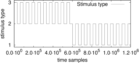
Figure 1: The manner in which stimuli were applied in the experiment. x-axis shows time samples and y-axis - stimulus types, where type 1 - right hand, 2 - no stimulus, 3 - left hand.

This somatosensory data set contained high frequency transient signals resulting from the electrical stimulus. These transients are distorted when filtered with a linear filter, due to ringing effects and adversely affect nearby data, including the expected early response at about 20ms post-stimulus. To avoid this and still be able to remove low frequency drifts, a median filter was used as follows. First, the signal was filtered with a median filter of window size set to obtain 1Hz low pass filter (1000 samples in our case). Second, the result from the previous step was subtracted from initial measurements to obtain 1Hz high-pass filtered signal. The large 60Hz noise and harmonics in the data were reduced but not removed by replacing the points in the power spectrum in the data near 60Hz and harmonics with values that interpolated between adjacent power spectrum points.

Noise samples of 35ms latency were extracted from the prestimulus area of right side stimulation no earlier than 300ms after the previous stimulus was applied. Since filtering can affect temporal covariance it is important to estimate covariance after filtering has been applied. All covariance models in this section were estimated using this continuous background data, scaled appropriately to obtain covariances of the noise averaged over 602 samples. All the covariance models yielded similar sensor variances, differences were only observed in the correlation structure.

Continuous noise samples were combined in a way that allowed for averaging over 602 independent samples. This approach supplied six different average noise data sets. Different signal to noise ratios (SNR) for single dipole problems were obtained by scaling these noise samples before combining them with simulated data. The measure of SNR used in this paper was constructed by squaring all values of the signal vector and then adding them together (inner product of the signal vector) and dividing this value by squared and summed values of the noise vector; a square root was taken from the obtained ratio.

The locations and orientations of fifty dipoles were drawn at random from the gray matter voxels that had been tagged from the subject’s anatomical MRI used in the empirical MEG experiment. In order to mitigate the effect of depth vs. strength that would complicate the interpretation of results, the area from which random locations were drawn was constrained to be further than five centimeters from the head center (Fig. 2).

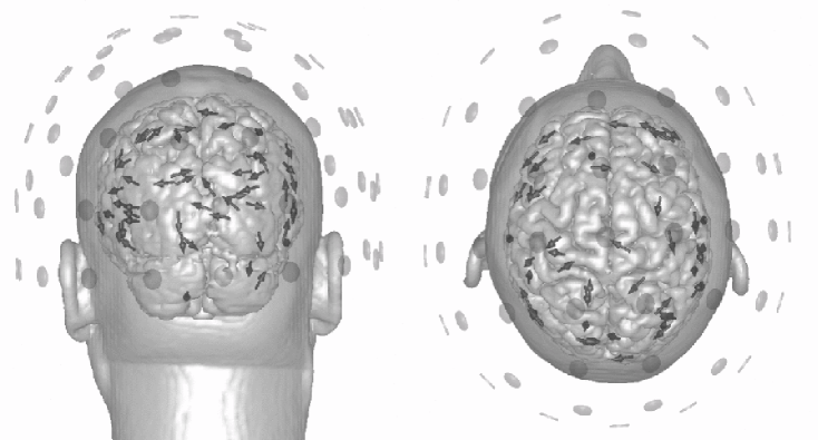
Figure 2: Dipoles randomly scattered over the cortex. These dipoles give fairly uniform coverage of the cortex and with different orientations create many possible realistic sources.

Each single dipole problem consisting of 121 sensor values over 35ms (121x35 matrix) was constructed in the following way:

1. For each dipole in the set of 50 a sinusoidal time course was used.

2. This dipole was projected to the sensor space using Sarvas’ spherical head model [30].

3. To the simulated signal one of the six noise sample sets was added. Noise was appropriately scaled in advance according to the intended SNR.

The total number of single dipole problems run through the inverse solution routine was 2400. This number combines 50 dipoles with 6 noise kinds for each and 8 SNR values (0.3,0.4,0.5,0.7,1.0,1.5,2.0,3.0). Figure 3 demonstrates how different the noise samples were and what diversity was introduced by changing SNR.

SNR 0.3		SNR 1.0	SNR 3.0

Figure 3: Three noise sample sets and three signal to noise ratios for one of the dipoles. Columns have the same signal to noise ratio and rows have the same noise instance added to the simulated dipole.

For each data set we estimated the location, orientation and time course of a single dipole that maximized the likelihood, using the different background covariance models. In these trials the location and orientation of the dipole did not vary over time. Initial attempts to solve for these parameters using an optimization algorithm were plagued by local minima problems, which is common in dipole inverse algorithms [31, 32]. The degree of these local minima errors confounded the errors between background covariance models. To mitigate this confound we employed a sampling algorithm using Markov Chain Monte Carlo (MCMC) [33, 34, 5], which sampled the location and orientation parameters from the likelihood using the maximum likelihood time course values for a given set of location and orientation parameters. From these samples we then calculated the mean values of the parameters and used this as our estimate of the maximum likelihood result. This reduced the local minima problems but did not eliminate them. To further reduce the local minima effects we ran multiple MCMC samplings for each data set and chose the results that had the highest likelihood. We are confident that the results from this set of procedures primarily reflect the errors associated with the different background covariance models.

There are 300 results for each SNR value for each model. Figure 4 shows a histogram of location errors for the diagonal model with SNR of 1.0. The shape of this distribution (non-Gaussian with large tails), is typical for all of the models and SNR values. From each of these distributions we calculated the point on the error axis below which 90% of the probability mass is concentrated. Figures 5(a) and 5(b) show these 90% error plots for location and time courses as a function of SNR for each background covariance model. Here the location error was calculated as the root mean squared error and the time course error was calculated as the root of the squared error averaged over time. The two multi-pair models had the lowest errors, followed by the two single pair models with slightly higher errors. Finally, the diagonal model had by far the largest errors.

Figure 4: Location error histogram for the case of using the diagonal covariance approximation at SNR 1.0

(a) location errors

(b) time course errors

Figure 5: Combined 90% location error measure 5(a) and combined 90% time course errors 5(b) for a series of single dipole problems.

4 Discussion

1
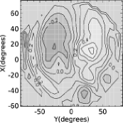
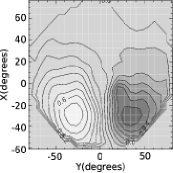
2
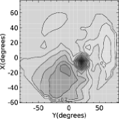
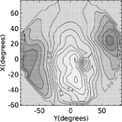
3
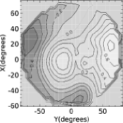
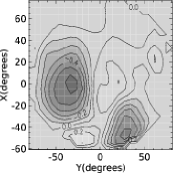
4
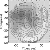
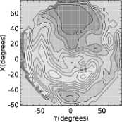
5
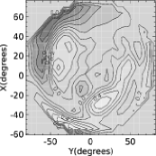
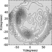
6
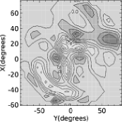
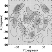
A		B	C	D

Figure 6: Contour plots of the first 10 the most significant spatial components with corresponding temporal covariance functions (above the line) and of 2 the least significant spatial components.

This work, like previous investigations, underscores the value of a suitable models of brain and other noise sources for accurate localization of neural sources. The most sophisticated models we tested gave the best performance, with improved estimation of both location and timecourse of the target neural source.

We also note the relatively small improvement in the multi-pair models over the single pair models. This is especially interesting given that the computational burden, both for estimating the parameters of the models and in implementing them in the inverse calculations, is relatively small for the single pair model and much higher for multi-pair models. Thus these findings suggest that a significant gain in performance may be had with a relatively small computational cost by using a single pair model. However, more work needs to be done to investigate the validity and generality of this finding. For example, these results are from a single subject, using single dipole sources and over a limited temporal range. Future work would investigate whether these results hold over multiple subjects, with more complex source configurations and for a more extended temporal range. It is possible that noise components will be more variable or more complex if these conditions change.

The assumption that each noise generator contributing to the measured background does not change its spatial location is supported by observations of stability of the brain function at the resting state [35]. Spatial diversity of the background signal can be observed, for example, as nonuniform spatial distribution of the alpha rhythm over the cortex. Moreover, the background may not have many generators with distinct independent time courses. In the data examined here the temporal covariances across components were relatively similar in the multi-pair models. This is a possible explanation of why the multi-pair models yield relatively little improvement over the single pair models.

Figure 6 shows contour plots of spatial components from the SVD based multi-pair model and their corresponding temporal covariances. There are clear differences among the temporal covariances. However, if one takes out the components that are either sensor dominated with very short temporal correlations (B2,B6 and D6) and the large 60% powerline component (B1) the remaining components, which are presumably dominated by background brain activity, have similar temporal correlation structure. It will be interesting to see if in future work this feature is observer across multiple subjects and over a more extended temporal range.

An observation was made in the course of this work that may support the supposition that our data does not exhibit great variability in the hidden source structure. The following heuristic was used to estimate one-pair Kronecker model for parallel comparison with the results presented in this paper. Suppose that each sensor has the same temporal covariance. Then it is possible to estimate the single-pair model using:

$$\hat{\mathbf{T}} = \frac{1}{M(LM-1)}\left(\mathbf{E}^{T}_{1},...\mathbf{E}^{T}_{M}\right)\left(\begin{array}[]{c}\mathbf{E}_{1}\\ \vdots\\ \mathbf{E}_{M}\end{array}\right)$$ (20)

$$\hat{\mathbf{S}} = \frac{1}{M(CM-1)}\left(\mathbf{E}_{1},...\mathbf{E}_{M}\right)\left(\begin{array}[]{c}\mathbf{E}^{T}_{1}\\ \vdots\\ \mathbf{E}^{T}_{M}\end{array}\right),$$ (24)

where $\mathbf{E}_{m}$ is an $L\times C$ single trial noise data with $L$ number of sensors and $C$ number of time points; $M$ is the number of trials. $\hat{\mathbf{T}}$ is normalized to leave the variances in $\hat{\mathbf{S}}$ only. This is not an optimized estimator, as compared to the single-pair Maximum Likelihood estimator; nevertheless, we found both of these estimators performed similarly. Looking at the two estimators, they could yield similar results if the structure of the noise is not very complicated. Furthermore, a compatible error might be introduced to the MLE based model when the assumption about the Gaussian distribution of the un-averaged measured background is violated.

Despite almost identical performance of the multi-pair models we suggest that in terms of generality the model based on independent basis should be preferred. Its power is not only in the increase of degrees of freedom and consequently the ability to describe a bigger class of possible spatial components but also in the discriminative criterion. The main criterion used in PCA is minimization of the reconstruction error [36]. As a result this produces spatially uncorrelated components. This may not be a good model of the MEG/EEG background, especially that due to the background brain activity. It seems more reasonable to assume that different noise generators are independent. In that case, the independent basis model is complex enough to describe the underlying process and a correct choice of algorithm (for example an ICA algorithm) can estimate independent generators.

Considering the observation that not all spatial components may have distinct temporal structure, a further generalization is needed. The multi-pair model can have an additional parameter for the number of significant components. In this case only significant components will contribute to the final covariance with their respective distinct time courses. Other components would be suppressed. This generalization is not obvious since special care should be taken to retain inversion of the model. We leave this work for subsequent publications.

Multi-pair models can in principle be directly applied to the analysis of EEG data. Though the topic needs further study it is expected that the different structure of EEG would not affect the multi-pair models as much as the possible added complexity of the noise. We expect that in the case of heterogeneous noise sources expected in EEG signals, multi-pair models should show even better performance due to their increased expressive power and ability to incorporate information about many noise components.

We also note that a further reduction of parameters for multi-pair models can be achieved by assuming stationarity of the background. This assumption is well supported by studies, see for example [37]. Observation of time courses of orthogonal and independent components for the data used in this study also supports this assumption. Temporal autocovariances have an Toeplitz-like structure and can be constructed from correlations shown in Figure 6. This assumption reduces the number of parameters to be estimated to $L(L+1)/2+LC$ for the SVD based model and to $L^{2}+LC$ for the ICA based model. Another important improvement this assumption provides is the reduction in running time for inverting the multi-pair approximations from $O(LC^{3})$ to $O(LC^{2})$ [38]. This will be investigated in future work.

Different models that would cover the range between the diagonal and the one-pair model can be developed. For such models an additional study is needed to investigate how spatial models alone or temporal models alone would compare in performance as well. These truncated models can be useful in the case when only a scarce amount of data is available for estimation. But when the single-pair model can be estimated it subsumes all lower order models and should not perform worse than these. As we show in this paper multi-pair models subsume the single-pair model and thus should not perform worse than it. This was demonstrated by the increased localization accuracy. In the case when sufficient estimation data is available and the additional computational load of multi-pair models does not make significant difference, we suggest using multi-pair models to increase accuracy. In the worst case, multi-pair models should not perform poorer than the one-pair model.

5 Conclusions

In this paper we have introduced two multi-pair spatiotemporal covariance models as a generalization over the previous work [2] which extends the expressive power and provides better localization results. The orthogonal basis multi-pair model estimated using SVD is a more general but still a restricted one due to the orthogonality constraints. A more general model is the independent basis multi-pair model estimated using an ICA algorithm. Models were compared on the basis of their performance in a localization algorithm. Performance statistics were gathered from inverse solutions to a large number of single dipole problems with simulated sources and background from real MEG data. In terms of localization error, the orthogonal basis and independent basis multi-pair models demonstrated the best performance. The independent basis model is a potentially better model due to the increase in the descriptive power. However, the errors from the single pair model examined were not much worse. Future work will address whether these findings are a general feature of MEG background across multiple subjects, with more complex source configurations and over a more extended temporal range.

Appendix A Derivation of multi-pair models

For the following derivation we need to calculate determinants of the multi-pair models. This is done in the Appendix C for the case of orthogonal basis model (53). Also the inverse of the orthogonal basis multi-pair model (13) is utilized in the following. Using these result the log likelihood for the Gaussian pdf for the orthogonal basis multi-pair model is expressed like:

$${\mathcal{L}}=const-\frac{M}{2}\sum_{l=1}^{L}\ln(|\bm{\mathcal{T}}^{l}|)-\frac{1}{2}tr(\sum_{m=1}^{M}\sum_{l=1}^{L}\mathbf{E}_{m}^{T}\bm{{\mathcal{S}}}^{l}\mathbf{E}_{m}(\bm{\mathcal{T}}^{l})^{-1})$$ (25)

Differentiating with respect to $\bm{\mathcal{T}}^{l}$ results in:

$$d{\mathcal{L}} = -\frac{M}{2}tr((\bm{\mathcal{T}}^{l})^{-1}d\bm{\mathcal{T}}^{l})+\frac{1}{2}tr(\sum_{m=1}^{M}\mathbf{E}_{m}^{T}\bm{{\mathcal{S}}}^{l}\mathbf{E}_{m}(\bm{\mathcal{T}}^{l})^{-1}d\bm{\mathcal{T}}^{l}(\bm{\mathcal{T}}^{l})^{-1})$$ (26)

$$= -\frac{M}{2}tr((\bm{\mathcal{T}}^{l})^{-1}d\bm{\mathcal{T}}^{l})+\frac{1}{2}tr(\sum_{m=1}^{M}(\bm{\mathcal{T}}^{l})^{-1}\mathbf{E}_{m}^{T}\bm{{\mathcal{S}}}^{l}\mathbf{E}_{m}(\bm{\mathcal{T}}^{l})^{-1}d\bm{\mathcal{T}}^{l})$$

$$= -\frac{M}{2}tr([(\bm{\mathcal{T}}^{l})^{-1}-\frac{1}{M}\sum_{m=1}^{M}(\bm{\mathcal{T}}^{l})^{-1}\mathbf{E}_{m}^{T}\bm{{\mathcal{S}}}^{l}\mathbf{E}_{m}(\bm{\mathcal{T}}^{l})^{-1}]d\bm{\mathcal{T}}^{l})$$

And the final result is:

$$\bm{\mathcal{T}}^{l}=\frac{1}{M}\sum_{m=1}^{M}\mathbf{E}_{m}^{T}\bm{{\mathcal{S}}}^{l}\mathbf{E}_{m}$$ (27)

Next we estimate temporal covariance for the independent basis multi-pair model. The determinant of the independent basis model is calculated in Appendix C equation (54) and the inverse of this model is taken as in (15). The log likelihood in this case:

$${\mathcal{L}} = const-\frac{M}{2}(2C\ln(|\mathbf{W}^{-1}|)+\sum_{l=1}^{L}\ln(|\bm{\mathcal{T}}^{l}|))$$ (28)

$$-\frac{1}{2}tr(\sum_{m=1}^{M}\sum_{l=1}^{L}\mathbf{E}_{m}^{T}\mathbf{WW}^{T}\bm{\mathcal{R}}^{l}\mathbf{WW}^{T}\mathbf{E}_{m}(\bm{\mathcal{T}}^{l})^{-1})$$

Following the same path for derivation as for the orthogonal basis model case we end up with:

$$\bm{\mathcal{T}}^{l}=\frac{1}{M}\sum_{m=1}^{M}\mathbf{E}_{m}^{T}\mathbf{WW}^{T}\bm{\mathcal{R}}^{l}\mathbf{WW}^{T}\mathbf{E}_{m}$$ (29)

Appendix B Inversion of the multi-pair models

We need the following identity for derivations of this section:

$$(\mathbf{A}_{1}\otimes\mathbf{B}_{1})(\mathbf{A}_{2}\otimes\mathbf{B}_{2})=(\mathbf{A}_{1}\mathbf{A}_{2}\otimes\mathbf{B}_{1}\mathbf{B}_{2})$$ (30)

First, lets prove that the inverse for the orthogonal basis multi-pair model is as in (13) . By the orthogonality of $\bm{{\mathcal{S}}}^{l}$ ($\bm{{\mathcal{S}}}^{l}\bm{{\mathcal{S}}}^{l^{\prime}}=0$ if $l\neq{l^{\prime}}$),

$$\widetilde{\mathbf{COV}}\ \widetilde{\mathbf{COV}}^{-1} = \left(\sum_{l=1}^{L}\lambda_{l}^{2}\bm{\mathcal{T}}^{l}\otimes\bm{{\mathcal{S}}}^{l}\right)\left(\sum_{l=1}^{L}\lambda_{l}^{-2}(\bm{\mathcal{T}}^{l})^{-1}\otimes\bm{{\mathcal{S}}}^{l}\right)$$ (31)

$$= \sum_{l=1}^{L}\mathbf{I}\otimes(\bm{{\mathcal{S}}}^{l})^{2}$$

By two properties of $\bm{{\mathcal{S}}}^{l}$: (1) $(\bm{{\mathcal{S}}}^{l})^{2}=\bm{{\mathcal{S}}}^{l}$; (2) $\sum_{l}\bm{{\mathcal{S}}}^{l}=\mathbf{I}$ due to orthogonality of $\mathbf{V}$, we obtain the desired one:

$$\widetilde{\mathbf{COV}}\ \widetilde{\mathbf{COV}}^{-1}=\sum_{l=1}^{L}\mathbf{I}\otimes(\bm{{\mathcal{S}}}^{l})^{2}=\mathbf{I}\otimes\sum_{l=1}^{L}\bm{{\mathcal{S}}}^{l}=\mathbf{I}\otimes\mathbf{I}=\mathbf{I}.$$ (32)

Properties of $\bm{{\mathcal{S}}}^{l}$ are proved as follows:

• property (1)

  $$(\bm{{\mathcal{S}}}^{l})^{2} = (v_{l}v_{l}^{T})(v_{l}v_{l}^{T})=v_{l}(v_{l}^{T}v_{l})v_{l}^{T}$$ (33)

  $$= v_{l}v_{l}^{T}\quad(v_{l}^{T}v_{l}=1\mbox{ by orthogonality of $\mathbf{V}$})$$

  $$= \bm{{\mathcal{S}}}^{l}$$

• property (2) : $\mathbf{I}=\mathbf{V}\ \mathbf{V}^{T}=\sum_{l}v_{l}v_{l}^{T}$

Now we show that the inverse of the independent components multi-pair model is as in (15) Using the identity (30)

$$\left(\sum_{l=1}^{L}\bm{\mathcal{T}}^{l}\otimes\bm{\mathcal{R}}^{l}\right)\left(\sum_{l=1}^{L}(\bm{\mathcal{T}}^{l})^{-1}\otimes[\mathbf{WW}^{T}\bm{\mathcal{R}}^{l}\mathbf{WW}^{T}]\right)$$

$$\quad=\sum_{l,l^{\prime}=1}^{L}\bm{\mathcal{T}}^{l}(\bm{\mathcal{T}}^{l^{\prime}})^{-1}\otimes[\bm{\mathcal{R}}^{l}\mathbf{WW}^{T}\bm{\mathcal{R}}^{l^{\prime}}\mathbf{WW}^{T}].$$ (34)

According to the definition of $\bm{\mathcal{R}}_{l}$:

$$\bm{\mathcal{R}}_{l}=w_{l}w_{l}^{T}=(\mathbf{W}^{-1})^{T}e_{l}e_{l}^{T}\mathbf{W}^{-1}.$$ (35)

Here $\{e_{l}|l=1,\cdots,L\}$ are orthonormal canonical bases vectors. By the orthogonality of $e_{l}$ and substituting (35) into (34), we obtain

$$\bm{\mathcal{R}}^{l}\mathbf{WW}^{T}\bm{\mathcal{R}}^{l^{\prime}}\mathbf{WW}^{T} = (\mathbf{W}^{-1})^{T}e_{l}e_{l}^{T}\mathbf{W}^{-1}\mathbf{WW}^{T}(\mathbf{W}^{-1})^{T}e_{l^{\prime}}e_{l^{\prime}}^{T}\mathbf{W}^{-1}\mathbf{WW}^{T}$$ (36)

$$= (\mathbf{W}^{-1})^{T}e_{l}e_{l}^{T}e_{l^{\prime}}e_{l^{\prime}}^{T}\mathbf{W}^{T}$$

$$= \delta(l,l^{\prime})(\mathbf{W}^{-1})^{T}e_{l}e_{l}^{T}\mathbf{W}^{T}$$

Finally, we obtain the desired result:

$$\left(\sum_{l=1}^{L}\bm{\mathcal{T}}^{l}\otimes\bm{\mathcal{R}}^{l}\right)\left(\sum_{l=1}^{L}(\bm{\mathcal{T}}^{l})^{-1}\otimes[\mathbf{WW}^{T}\bm{\mathcal{R}}^{l}\mathbf{WW}^{T}]\right)$$

$$\quad=\mathbf{I}\otimes(\mathbf{W}^{-1})^{T}[\sum_{l}e_{l}e_{l}^{T}]\mathbf{W}^{T}=\mathbf{I}\otimes(\mathbf{W}^{-1})^{T}\mathbf{I}\mathbf{W}^{T}=\mathbf{I}.$$ (37)

Appendix C Calculation of the determinant

Before performing actual calculations of the determinant we transfrom the original series form to a shape more manageable in our further reasoning. The only assumption needed for the transformation is that matrices $S^{l}$ are rank one outer products $v_{l}v_{l}^{T}$, where $v_{l}$ comes from an independent basis set.

We first rewrite $\displaystyle\sum T^{l}\otimes S^{l}$ in the matrix form:

$$\sum T^{l}\otimes S^{l}=\left[\begin{array}[]{cccc}\sum_{l=1}^{L}T^{l}_{1,1}S^{l}&\sum_{l=1}^{L}T^{l}_{1,2}S^{l}&\cdots&\sum_{l=1}^{L}T^{l}_{1,C}S^{l}\\ \sum_{l=1}^{L}T^{l}_{2,1}S^{l}&\sum_{l=1}^{L}T^{l}_{2,2}S^{l}&\cdots&\sum_{l=1}^{L}T^{l}_{2,C}S^{l}\\ \vdots&\vdots&\ddots&\vdots\\ \sum_{l=1}^{L}T^{l}_{C,1}S^{l}&\sum_{l=1}^{L}T^{l}_{C,2}S^{l}&\cdots&\sum_{l=1}^{L}T^{l}_{C,C}S^{l}\\ \end{array}\right]$$ (38)

Considering each element separately we can see that:

$$\sum_{l=1}^{L}T^{l}_{i,j}S^{l}=\sum_{l=1}^{L}T^{l}_{i,j}v_{l}v_{l}^{T}=S\Lambda_{i,j}S^{T},$$ (39)

where $S$ is an $L\times L$ matrix with columns being $v_{l}$ vectors from an orthonormal basis; $\Lambda_{i,j}$ is a diagonal matrix with the elements along the diagonal being $\{T^{1}_{i,j},T^{2}_{i,j},\ldots,T^{L}_{i,j}\}$. Observing (39) one more rewrite is possible:

$$\sum T^{l}\otimes S^{l}=\left[\begin{array}[]{cccc}S&0&\cdots&0\\ 0&S&\cdots&0\\ \vdots&\vdots&\ddots&\vdots\\ 0&0&\cdots&S\\ \end{array}\right]\left[\begin{array}[]{cccc}\Lambda_{1,1}&\Lambda_{1,2}&\cdots&\Lambda_{1,C}\\ \Lambda_{2,1}&\Lambda_{2,2}&\cdots&\Lambda_{2,C}\\ \vdots&\vdots&\ddots&\vdots\\ \Lambda_{C,1}&\Lambda_{C,2}&\cdots&\Lambda_{C,C}\\ \end{array}\right]\left[\begin{array}[]{cccc}S^{T}&0&\cdots&0\\ 0&S^{T}&\cdots&0\\ \vdots&\vdots&\ddots&\vdots\\ 0&0&\cdots&S^{T}\\ \end{array}\right]$$ (40)

The next step is actually calculating the determinant $\det\left(\displaystyle\sum T^{l}\otimes S^{l}\right)$:

$$\det\left(\left[\begin{array}[]{cccc}S&0&\cdots&0\\ 0&S&\cdots&0\\ \vdots&\vdots&\ddots&\vdots\\ 0&0&\cdots&S\\ \end{array}\right]\right)\det\left(\left[\begin{array}[]{cccc}\Lambda_{1,1}&\Lambda_{1,2}&\cdots&\Lambda_{1,C}\\ \Lambda_{2,1}&\Lambda_{2,2}&\cdots&\Lambda_{2,C}\\ \vdots&\vdots&\ddots&\vdots\\ \Lambda_{C,1}&\Lambda_{C,2}&\cdots&\Lambda_{C,C}\\ \end{array}\right]\right)\det\left(\left[\begin{array}[]{cccc}S^{T}&0&\cdots&0\\ 0&S^{T}&\cdots&0\\ \vdots&\vdots&\ddots&\vdots\\ 0&0&\cdots&S^{T}\\ \end{array}\right]\right)$$ (41)

Let’s leave diagonal matrices alone since their determinants are trivial and calculate the middle determinant. Let’s introduce $E^{l}=e_{l}e_{l}^{T}$, where $e_{l}$ is a basis vector from the canonical basis set. Now the matrix of ${\Lambda_{i,j}}$ can be consequently rewritten as:

$$\sum_{l=1}^{L}T^{l}\otimes E^{l}=\left[\begin{array}[]{cccc}\sum_{l=1}^{L}T^{l}_{1,1}E^{l}&\sum_{l=1}^{L}T^{l}_{1,2}E^{l}&\cdots&\sum_{l=1}^{L}T^{l}_{1,C}E^{l}\\ \sum_{l=1}^{L}T^{l}_{2,1}E^{l}&\sum_{l=1}^{L}T^{l}_{2,2}E^{l}&\cdots&\sum_{l=1}^{L}T^{l}_{2,C}E^{l}\\ \vdots&\vdots&\ddots&\vdots\\ \sum_{l=1}^{L}T^{l}_{C,1}E^{l}&\sum_{l=1}^{L}T^{l}_{C,2}E^{l}&\cdots&\sum_{l=1}^{L}T^{l}_{C,C}E^{l}\\ \end{array}\right]$$ (42)

By definition the determinant of a $C\times C$ matrix $A$ is:

$$\det(A)=\sum_{\rho}\sigma(\rho)a_{1,\rho_{1}}a_{1,\rho_{2}}\ldots a_{1,\rho_{C}},$$ (43)

where $\rho$ is a permutation, $\sigma(\rho)$ is the sign of a permutation and $a_{i,j}$ is an element of $A$.

Because of the orthogonality of $E^{l}$ matrices to each other when their indices are not the same and using the property $(E^{l})^{n}=E^{l}$:

$$\det\left(\displaystyle\sum_{l=1}^{L}T^{l}\otimes E^{l}\right) = \det\left(\displaystyle\sum_{\rho}\sigma(\rho)\displaystyle\sum_{l}T^{l}_{1,\rho_{1}}T^{l}_{1,\rho_{2}}\ldots T^{l}_{1,\rho_{C}}E^{l}\right)$$ (44)

$$\det\left(\displaystyle\sum_{l=1}^{L}T^{l}\otimes E^{l}\right) = \det\left(\displaystyle\sum_{l}\left(\displaystyle\sum_{\rho}\sigma(\rho)T^{l}_{1,\rho_{1}}T^{l}_{1,\rho_{2}}\ldots T^{l}_{1,\rho_{C}}\right)E^{l}\right)$$ (45)

$$\det\left(\displaystyle\sum_{l=1}^{L}T^{l}\otimes E^{l}\right) = \det\left(\displaystyle\sum_{l}\det\left(T^{l}\right)E^{l}\right)$$ (46)

$$\det\left(\displaystyle\sum_{l=1}^{L}T^{l}\otimes E^{l}\right) = \det\left(I\left[\begin{array}[]{ccc}\ddots&&0\\ &\det\left(T^{l}\right)&\\ 0&&\ddots\\ \end{array}\right]I\right)$$ (50)

$$\det\left(\displaystyle\sum_{l=1}^{L}T^{l}\otimes E^{l}\right) = \displaystyle\prod_{l}^{L}\det\left(T^{l}\right)$$ (51)

With this result (51) the determinant from (41) can be rewritten:

$$\det\left(\displaystyle\sum T^{l}\otimes S^{l}\right)=\det\left(S\right)^{2C}\displaystyle\prod_{l}^{L}\det\left(T^{l}\right)$$ (52)

We first calculate a special case when $\bm{\mathcal{S}}^{l}=v_{l}v_{l}^{T}$ and all column vectors $v_{l}$ belong to an orthonormal basis, that is $S$ from (52) in an orthogonal matrix. In this case $\det(S)=1$ and the result is:

$$\det\left(\displaystyle\sum T^{l}\otimes S^{l}\right)=\displaystyle\prod_{l}^{L}\det\left(T^{l}\right)$$ (53)

In the case when $S$ is not orthogonal like in the ICA case, we get slightly different result. Redefine $S^{l}=R^{l}$, where $R^{l}=w_{l}w_{l}^{T}$ and $w_{l}$ is a row vector of the mixing matrix $W^{-1}$. Then (52) becomes:

$$\det\left(\displaystyle\sum T^{l}\otimes R^{l}\right)=\det\left(W^{-1}\right)^{2C}\displaystyle\prod_{l}^{L}\det\left(T^{l}\right)$$ (54)

References

- [1] H. M. Huizenga, J. C. De Munck, L. J. Waldorp, R. P. Grasman, Spatiotemporal EEG/MEG source analysis based on a parametric noise covariance model, IEEE Trans Biomed. Engin. 50 (2002) 533–539.
- [2] J. C. De Munck, H. M. Huizenga, L. J. Waldorp, R. Heethaar, Estimating stationary dipoles from MEG/EEG data contaminated with spatially and temporally correlated background noise, IEEE Transaction on Signal Processing 50 (7) (2002) 1565–1572.
- [3] M. Hämäläinen, R. Hari, R. Ilmoniemi, J. Knuutila, O. Lounasmaa, Magnetoencephalography: theory, instrumentation, and applications to noninvasive studies of the working human brain, Rev. Mod. Phys. 65 (1993) 413–497.
- [4] J. C. Mosher, P. S. Lewis, R. M. Leahy, Multiple dipole modeling and localization from spatio-temporal meg data., IEEE transactions on bio-medical engineering 39 (6) (1992) 541 – 57.
- [5] D. M. Schmidt, J. S. George, C. C. Wood, Bayesian inference applied to the electromagnetic inverse problem, Human Brain Mapping 7 (1999) 195–212.
- [6] J. W. Phillips, R. M. Leahy, J. C. Mosher, MEG-based imaging of focal neuronal current sources, IEEE Trans. Med. Imag. 16 (1997) 338–348.
- [7] B. D. VanVeen, W. vanDrongelen, M. Yuchtman, A. Suzuki, Localization of brain electrical activity via linearly constrained minimum variance spatial filtering., IEEE transactions on bio-medical engineering 44 (9) (1997) 867 – 80.
- [8] M. Hämäläinen, R. Ilmoniemi, Interpreting magnetic fields of the brain: minimum norm estimates., Med Biol Eng Comput 32 (1) (1994) 35–42.
- [9] S. Kuriki, F. Takeuchi, T. Kobayashi, Characteristics of the background fields in multichannel-recorded magnetic field responses., Electroencephalography and clinical neurophysiology evoked potentials 92 (1994) 56–63.
- [10] H. Huizenga, P. Molenaar, Ordinary least squares dipole localization is influenced by the reference, Electroencephalography and clinical neurophysiology 99 (1996) 562–567.
- [11] B. Lutkenhoner, Dipole source localization by means of maximum likelihood estimation. II. Experimental evaluation., Electroencephalogr Clin Neurophysiol 106 (4) (1998) 322–9.
- [12] S. C. Jun, B. A. Pearlmutter, G. Nolte, Fast accurate MEG source localization using a multilayer perc eptron trained with real brain noise, Physics in Medicine and Biology 47 (14) (2002) 2547–2560.
- [13] V. Strassen, Gaussian elimination is not optimal, Numerische Mathematik 13 (4) (1969) 354.
- [14] D. Coppersmith, S. Winograd, Matrix multiplication via arithmetic progressions, Journal of Symbolic Computation 9 (3) (1990) 251–80.
- [15] J. H. H. L. K. Saul, K. Q. Weinberger, Semisupervised Learning, MIT Press: Cambridge, MA, 2005, to be published.
- [16] R. Vigario, J. Sarela, V. Jousmaki, M. Hamalainen, E. Oja, Independent component approach to the analysis of EEG and MEG recordings., IEEE Trans Biomed Eng 47 (5) (2000) 589–93.
- [17] A. Tang, B. Pearlmutter, N. Malaszenko, D. Phung, B. Reeb, Independent components of magnetoencephalography: localization., Neural Comput 14 (8) (2002) 1827–58.
- [18] A. Tang, B. Pearlmutter, N. Malaszenko, D. Phung, Independent components of magnetoencephalography: single-trial response onset times., Neuroimage 17 (4) (2002) 1773–89.
- [19] A. Ziehe, K. Muller, G. Nolte, B. Mackert, G. Curio, Artifact reduction in magnetoneurography based on time-delayed second-order correlations., IEEE Trans Biomed Eng 47 (1) (2000) 75–87.
- [20] J. Cao, N. Murata, S. Amari, A. Cichocki, T. Takeda, H. Endo, N. Harada, Single-trial magnetoencephalographic data decomposition and localization based on independent component analysis approach, IEICE Transactions on Fundamentals of Electronics, Communications and Computer Sciences E83-A (9) (2000) 1757–1766.
- [21] S. Makeig, T. Jung, A. Bell, D. Ghahremani, T. Sejnowski, Blind separation of auditory event-related brain responses into independent components., Proc Natl Acad Sci U S A 94 (20) (1997) 10979–84.
- [22] S. Makeig, M. Westerfield, T. Jung, J. Covington, J. Townsend, T. Sejnowski, E. Courchesne, Functionally independent components of the late positive event-related potential during visual spatial attention., J Neurosci 19 (7) (1999) 2665–80.
- [23] T. Jung, S. Makeig, C. Humphries, T. Lee, M. McKeown, V. Iragui, T. Sejnowski, Removing electroencephalographic artifacts by blind source separation., Psychophysiology 37 (2) (2000) 163–78.
- [24] A. Belouchrani, K. Abed Meraim, J.-F. Cardoso, Éric Moulines, Second-order blind separation of correlated sources, in: Proc. Int. Conf. on Digital Sig. Proc., Cyprus, 1993, pp. 346–351.
- [25] A. J. Bell, T. J. Sejnowski, An information-maximization approach to blind separation and blind deconvolution, Neural Computation 7 (1995) 1129–1159.
- [26] A. Hyvärinen, E. Oja, A fast fixed-point algorithm for independent component analysis, Neural computation 9 (7) (1997) 1483–1492.
-
[27]
A. Cichocki, S. Amari, K. Siwek, ICALAB Toolboxes.
URL http://www.bsp.brain.riken.jp/ICALAB - [28] S. Kullback, R. A. Leibler, On information and sufficiency, Ann. Math. Stat. 22 (1951) 79–86.
- [29] A. Ahonen, M. Hamalainen, M. Kajola, J. Knuutila, P. Laine, O. Lounasmaa, L. Parkkonen, J. Simola, C. Tesche, 122-channel SQUID instrument for investigating the magnetic signals from the Human brain, Physica scripta T49A (1993) 198–205.
- [30] J. Sarvas, Basic mathematical and electromagnetic concepts of the biomagnetic inverse problem., Phys Med Biol 32 (1) (1987) 11–22.
- [31] Huang M, Aine CJ, Supek S, Best E, Ranken D, Flynn ER., Multi-start downhill simplex method for spatio-temporal source localization in magnetoencephalography, Electroenceph Clin Neurophysiol 108 (1) (1998) 32–44.
-
[32]
Ranken D, Best E, Stephen J, D. Schmidt, George J, Wood CC, Huang
MX, MEG/EEG Forward and inverse modeling using MRIVIEW, in: Biomag
2002 Proceedings, 2002, pp. 785–787.
URL http://www.lanl.gov/p/p21/mriview.shtml - [33] A. Gelman, J. B. Carlin, H. S. Stern, D. B. Rubin, Bayesian Data Analysis, Chapman & Hall, London, 1995.
- [34] S. C. Jun, J. S. George, J. Pare-Blagoev, S. Plis, D. M. Ranken, D. M. Schmidt, C. C. Wood, Spatiotemporal bayesian inference dipole analysis for MEG neuroimaging data, Neuroimage 28 (2005) 84–98.
- [35] M. E. Raichle, A. M. MacLeod, A. Z. Snyder, W. J. Powers, D. A. Gusnard, G. L. Shulman, A default mode of brain function., Proceedings of the National Academy of Sciences of the United States of America 98 (2) (2001) 676 – 682.
- [36] J. J. Gerbrands, On the relationships between svd, klt and pca., Pattern recognition 14 (1-6) (1980) 375 – 81.
- [37] F. Bijma, J. de Munck, H. Huizenga, R. Heethaar, A mathematical approach to the temporal stationarity of background noise in MEG/EEG measurements., Neuroimage 20 (1) (2003) 233–43.
- [38] R. E. Blahut, Fast Algorithms for Digital Signal Processing, Addison-Wesley, Reading, MA, USA, 1985.