Power-law distributions in economics: a nonextensive statistical approach

Abstract

The cornerstone of Boltzmann-Gibbs ($BG$) statistical mechanics is the Boltzmann-Gibbs-Jaynes-Shannon entropy $S_{BG}\equiv-k\int dx\,f(x)\ln f(x)$, where $k$ is a positive constant and $f(x)$ a probability density function. This theory has exibited, along more than one century, great success in the treatment of systems where short spatio/temporal correlations dominate. There are, however, anomalous natural and artificial systems that violate the basic requirements for its applicability. Different physical entropies, other than the standard one, appear to be necessary in order to satisfactorily deal with such anomalies. One of such entropies is $S_{q}\equiv k\,(1-\int dx\,[f(x)]^{q})/(1-q)$ (with $S_{1}=S_{BG}$), where the entropic index $q$ is a real parameter. It has been proposed as the basis for a generalization, referred to as nonextensive statistical mechanics, of the $BG$ theory. $S_{q}$ shares with $S_{BG}$ four remarkable properties, namely concavity ($\forall q>0$), Lesche-stability ($\forall q>0$), finiteness of the entropy production per unit time ($q\in\Re$), and additivity (for at least a compact support of $q$ including $q=1$). The simultaneous validity of these properties suggests that $S_{q}$ is appropriate for bridging, at a macroscopic level, with classical thermodynamics itself. In the same natural way that exponential probability functions arise in the standard context, power-law tailed distributions, even with exponents out of the Lévy range, arise in the nonextensive framework. In this review, we intend to show that many processes of interest in economy, for which fat-tailed probability functions are empirically observed, can be described in terms of the statistical mechanisms that underly the nonextensive theory.

I Introduction

The concept of “entropy” (from the greek $\tau\rho o\pi\acute{\eta}$, transformation), was introduced in $1865$ by Rudolf Julius Emmanuel Clausius in the context of Thermodynamicsfermi . This was motivated by his studies on reversible and irreversible transformations, as a measure of the amount of energy in a physical system, that cannot be used to perform work. More specifically, Clausius defined change in entropy of a thermodynamic system, during some reversible process where a certain amount of heat $\delta Q$ is transported at constant temperature $T$, as $\delta S=\delta Q/T$. We can consider entropy as the cornerstone of Thermodynamics, since all the thermodynamical principles involve, directly or indirectly, this fundamental concept.

The first connection between the macroscopic Clausius’ entropy of a system and its microscopic configurations was done by Ludwig Boltzmann in $1877$ fermi . Studying the approach to equilibrium of an “ideal” gas boltz , he realized that the entropy could be related to the number of possible microstates compatible with the thermodynamic properties of the gas. For an isolated system in its terminal stationary state (thermal equilibrium), Boltzmann observation can be expressed as

$$S_{BG}=k\,\ln W,$$ (1)

where $k$ is a positive constant and $W$ the number of microstates consistent with the macroscopic state. This famous equation, known as Boltzmann principle, can be regarded as a pillar in the foundations of statistical mechanics, which aims to describe the thermodynamic state of a system through the statistical approach of its microstates.

For systems which are not isolated but instead are in contact with some reservoir (of heat, particles, etc.), it is possible to derive (under some assumptions), from Eq. (1)   SBG , the celebrated Boltzmann-Gibbs entropy

$$S_{BG}=-k\sum\limits_{i=1}^{W}p_{i}\,\ln p_{i},$$ (2)

where $p_{i}$, subject to the normalization condition $\sum_{i=1}^{W}p_{i}=1$, is the probability of the microscopic configuration $i$. In particular, for equiprobability, $p_{i}=1/W$, $\forall_{i}$, then Boltzmann-Gibbs entropy (2) reduces to (1). Since it refers to microscopic states, the Boltzmann principle should be derivable from microscopic dynamics. However, the implementation of such calculation has not been yet achieved. Consequently, $BG$ statistical mechanics still remains based on hypothesis such as Boltzmann’s Stosszahlansatz (molecular chaos hypothesis)boltz and ergodicity khinchin . It can be easily shown that entropy (2) is nonnegative, concave, experimentally robust (or Lesche-stable)SBG ; props , and leads to a finite entropy production per unit timelatorabaranger99 . Moreover, it is additive. In other words, if $A$ and $B$ are two probabilistically independent subsystems, i.e., $p_{ij}^{A+B}=p_{i}^{A}p_{j}^{B}$, then it is straightforwardly verified that

$$S_{BG}\left(A+B\right)=S_{BG}\left(A\right)+S_{BG}\left(B\right),$$

hence, if we have $N$ subsystems, $S_{BG}(N)=NS_{BG}(1)$, where the notation is self-explanatory. More generally, when correlations are “weak” enough, $S_{BG}$ is extensive, i.e., such that the $\lim_{N\rightarrow\infty}S_{BG}(N)/N$ is finite.

Despite the lack of first-principle derivations, Boltzmann-Gibbs statistical mechanics has a history plenty of successes in the treatment of systems where short spatio/temporal interactions dominate. This kind of interactions favor ergodicity and independence properties, necessary in Khinchin’s approach of $S_{BG}$ khinchin . Consequently, it is perfectly plausible that physical entropies other than the Boltzmann-Gibbs one can be defined in order to suitably treat anomalous systems, for which ergodicity and/or independence are not verified. As examples of anomalies we can mention: metastable states in long-range interacting Hamiltonian systems, metaequilibrium states in small systems (i.e., systems whose number of particles is much smaller than Avogrado’s number), glassy systems, some types of dissipative systems, systems that in some way violate ergodicity, and, last but not least, systems with non-Markovian memory, like it seems to be the case of financial ones. Generically speaking, systems that may possibly have a multifractal, scale-free or hierarchical structure in the occupancy of their phase space.

Motivated by this scenario, one of us proposed in $1988$ the entropyct88

$$S_{q}=k\frac{1-\sum\limits_{i=1}^{W}p_{i}^{q}}{1-q}\qquad\left(q\in\Re\right),$$ (3)

which generalizes $S_{BG}$, such that $\lim_{q\rightarrow 1}S_{q}=S_{BG}$, as the basis of a possible generalization of Boltzmann-Gibbs statistical mechanicsfurther and where the entropic index $q$ should be determined a priori from microscopic dynamics. Just like $S_{BG}$, $S_{q}$ is nonnegative, concave, experimentally robust (or Lesche-stable) ($\forall{q>0}$), and leads to a finite entropy production per unit time (qprops and references therein). Moreover, it has been recently shownadditive that it is also additive, i.e.,

$$S_{q}\left(A_{1}+A_{2}+\ldots+A_{N}\right)=\sum\limits_{i=1}^{N}S_{q}\left(A_{i}\right),$$

for special kinds of correlated systems, more precisley when phase-space is occupied in a scale-invariant form.

Since its proposal, entropy (3) has been the source of numerous results in both fundamental and applied physics as well as in other scientific areas such as biology, chemistry, economics, geophysics and medicine applications . It is our purpose here to review some new results concerning applications to economics and more specifically to the theory of finances.

II Probability density functions from the variational principle

Before discussing some specific quantities of financial interest, let us see the form of the probability density function naturally derived from the variational principle related to entropy (3). We consider its continuous version, i.e.,

$$S_{q}=k\frac{1-\int\left[p\left(x\right)\right]^{q}\ dx}{1-q}.$$ (4)

Natural constraints in the maximization of (4) are

$$\int p\left(x\right)\ dx=1\,,$$

corresponding to normalization, and

$$\int x\frac{\ \left[p\left(x\right)\right]^{q}}{\int\left[p\left(x\right)\right]^{q}dx}\ dx\equiv\left\langle x\right\rangle_{q}=\bar{\mu}_{q}\,,$$ (5)

$$\int\left(x-\bar{\mu}_{q}\right)^{2}\frac{\ \left[p\left(x\right)\right]^{q}}{\int\left[p\left(x\right)\right]^{q}dx}\ dx\equiv\left\langle\left(x-\bar{\mu}_{q}\right)^{2}\right\rangle_{q}=\bar{\sigma}_{q}^{2}\,,$$ (6)

corresponding to the generalized mean and variance of a relevant quantity $x$, respectively. It is noteworthy that, averages weighted with a function of the probabilities as in (5)-(6) allow to mimic the way individuals behave in face to risky choicesrisk (see also also ). In fact, the prospect theory proposed by Kahneman and Tverskyat1 for analyzing decision-making under risk, is founded on the concept of “decision weights” that can be modeled by akin functional formsshape .

From the variational problem for (4) under the above constraints, one obtains

$$p\left(x\right)=\mathcal{A}_{q}\left[1+\left(q-1\right)\mathcal{B}_{q}\left(x-\bar{\mu}_{q}\right)^{2}\right]^{\frac{1}{1-q}},\qquad\left(q<3\right),$$ (7)

where,

$$\mathcal{A}_{q}=\left\{\begin{array}[]{ccc}\frac{\Gamma\left[\frac{5-3q}{2-2q}\right]}{\Gamma\left[\frac{2-q}{1-q}\right]}\sqrt{\frac{1-q}{\pi}\mathcal{B}_{q}}&\Leftarrow&q<1\\[8.53581pt] \frac{\Gamma\left[\frac{1}{q-1}\right]}{\Gamma\left[\frac{3-q}{2q-2}\right]}\sqrt{\frac{q-1}{\pi}\mathcal{B}_{q}}&\Leftarrow&q>1\end{array}\right.,$$

and

$$\mathcal{B}_{q}=\left[\left(3-1\right)\,\bar{\sigma}_{q}^{2}\right]^{-1}.$$

The upper bound $q=3$ guarantees normalizability. Defining the $q$-exponential function as

$$e_{q}^{x}\equiv\left[1+\left(1-q\right)\,x\right]^{\frac{1}{1-q}}\qquad\left(e_{1}^{x}\equiv e^{x}\right),$$

($e_{q}^{x}=0$ if $1+(1-q)x\leq 0$) we can rewrite the probability density (7) as

$$p\left(x\right)=\mathcal{A}_{q}\,e_{q}^{-\mathcal{B}_{q}\left(x-\bar{\mu}_{q}\right)^{2}},$$ (8)

hereon referred to as $q$-Gaussian probability density function.

For $q=\frac{3+m}{1+m}$, the $q$-Gaussian form recovers the Student’s $t$-distribution with $m$ degrees of freedom ($m=1,2,3,\ldots$). Consistently, for $q>1,$ (8) presents an asymptotic power-law behavior. Also, if $q=\frac{n-4}{n-2}$ with $n=3,4,5,\ldots$,  $p\left(x\right)$ recovers the $r$-distribution with $n$ degrees of freedom. Consistently, for $q<1$, $p\left(x\right)$ has a compact support which is defined by the condition $\left|x-\bar{\mu}_{q}\right|\leq\sqrt{\frac{3-q}{1-q}\,\bar{\sigma}_{q}^{2}}$.

Many other entropic forms have been introduced in the literature for various interesting purposes. One of the advantages of entropy (3) is that it yields power-law tails, which play a particularly relevant role, as well known.

Let us recall succinctly the two basic central limit theorems: (1) A convoluted distribution with a finite second moment approaches, in the limit of $N\to\infty$ convolutions, a Gaussian attractor; (2) A convoluted distribution with a divergent second moment, approaches, in the same limit, a Lévy distribution $L_{\gamma}(x)$ (with $0<\gamma<2$)andre . However, through dynamics different from the convolution one, for instance with some sort of memory across successive steps (i.e., nonindependence of the successive distributions), different ubiquitous distributions might arise (see also additive ). If the Laplacian term in the linear diffusion equation is a standard second derivative or a fractional derivative, the Gaussian or the Lévy distributions are respectively attained as solutions. However, much more complex and rich dynamics clearly exist in nature, for example those associated with a variety of nonlinear Fokker-Planck equations involving nontrivial correlations, multiplicative noise or other effects, as we will see in the following Section. Moreover, simple convolutions allow only for asymptotic behavior like the $q=1$ (Gaussian) or $q>5/3$ (Lévy distributions) ones. But they do not allow fat-tailed distributions associated with $1<q\leq 5/3$. However, many complex systems in nature as well as in social sciences exhibit exponents which precisely belong to that interval. An example of financial interest is exhibited in Fig 1.

Figure 1: Probability density function of returns, $P(r)$, versus return, $r$. The symbols represent $P(r)$ for the Dow Jones Industrial daily return index from 1900 until 2003. The solid line represents the best q-Gaussian numerical adjust with $q=1.54$ and $\sigma_{q}^{2}=0.338$ (as obtained in smdq-quantf ) and the dashed line a Gaussian fit.

III Underlying stochastic processes

The Gaussian distribution, recovered in the limit $q\rightarrow 1$ of expression (8), can be derived on a variety of grounds. For instance, it has been derived, through arguments based on the dynamics, by L. Bachelier in his 1900 work on price changes in Paris stock market, and also by A. Einstein in his 1905 article on Brownian motion. In particular, starting from a Langevin dynamics, one is able to write the corresponding Fokker-Planck equation and, from it, to obtain as solution the Gaussian distribution. Analogously, it is also possible, from certain classes of stochastic differential equations and their associated Fokker-Planck equations, to obtain the distribution given by (8).

In this section we will discuss dynamical mechanisms which lead to probability functions with asymptotic power-law behavior of the $q$-Gaussian form.

III.1 Stochastic processes with additive multiplicative structure

Microscopic dynamics containing multiplicative noise may be encountered in many dynamical processes and, due to its significance, has been the subject of numerous studies in the last decades. The presence of additive noise, besides the multiplicative contribution, is in fact a quite realistic ingredient since not all the fluctuations are processed multiplicatively. In previous workmulti1 , we considered a class of differential stochastic equations of the form

$$\dot{x}\;=\;f(x)+g(x)\zeta(t)\;+\;\eta(t)\,,$$ (9)

where $f,g$ are arbitrary functions of the stochastic variable $x$, and $\zeta(t),\eta(t)$, two independent zero-mean Gaussian white noises with variance $M^{2}$ and $A^{2}$, respectively. We have shown that for special forms of the deterministic force, namely $f(x)=-\gamma g(x)g^{\prime}(x)$, the stationary probability density functions (by using the Itô prescription) are of the form

$$P_{s}(x)\propto e_{q}^{-\beta[g(x)]^{2}}\,,$$ (10)

where $\beta\equiv(\gamma+M^{2})/A^{2}$ and

$$q\;=\;\frac{1+2M^{2}/\gamma}{1+M^{2}/\gamma}\,.$$ (11)

From the point of view of entropy $S_{q}$, the density function (10) derives from the variational principle, under the constraints of normalization and generalized variance of $g(u)$.

In particular, $q$-Gaussian distributions can be derived from a stochastic process of the linear formmulti1 ; multi2 ; multi3 ; multi4

$$\dot{x}\;=\;-\gamma x+x\zeta(t)\;+\;\eta(t)\,.$$ (12)

In fact, its associated Fokker-Planck equation is

$$\frac{\partial P}{\partial t}=\gamma\frac{\partial(xP)}{\partial x}+\frac{A^{2}}{2}\frac{\partial^{2}[(1+(M/A)^{2}x^{2})P]}{\partial x^{2}}$$ (13)

that has the alternative form

$$\frac{\partial P}{\partial t}=\gamma\frac{\partial(xP)}{\partial x}+\frac{D}{2}\frac{\partial P^{\nu}}{\partial x^{2}}\,,$$ (14)

where $\nu=2-q$, and $D$ is a constant related to the other model parameters. Eq. (14) is a nonlinear diffusion equation, familiarly known as porous media equation. Its steady state solution has the form

$$P_{s}(x)\propto e_{q}^{-\beta x^{2}}\,$$ (15)

with $q$ and $\beta$ defined as above. In the particular case $\nu=1=q$ the standard Gaussian steady state is obtained, corresponding to a purely additive process.

Taking into account that empirical returns where found to follow a $q$-Gaussian distributionlisa (see also Fig. 1), Eq. (12), complemented by the Itô prescription, provides a simple mechanism to model the dynamics of prices. Along similar lines it has been worked out, for instance, an option-pricing model which is more realistic than the celebrated Black-Scholes onelisa (recovered as the $q=1$ particular case).

The $q$-exponential character of the solutions of Eq. (14) is not exclusive of the steady state but it also emerges along the time evolutionmulti1 ; FP_nl . In the presence of multiplicative noise, the system variables directly couple to noise. Therefore, behaviors are observed that can not occur in the presence of additive noise alone. On the other hand the additive noise plays a fundamental role allowing the existence of a reasonable and normalizable steady state by avoiding collapse of the distribution at the origin. The particular interplay between additive and multiplicative noises, as well as that between deterministic and stochastic drifts, can lead to the appearance of $q$-exponential forms.

The $q$-exponential distributions include the Boltzmann-Gibbs one as a special case ($q=1$). While the latter corresponds to the standard thermal equilibrium, the $q\neq 1$ is expected to be related to quasi-stationary or long-living out-of-equilibrium regimes.

III.2 Stochastic processes with varying intensive parameters

Intricate dynamical behavior is a common feature of many non-equilibrium systems, which can be also characterized by power-law probability density functions. To this class belong systems whose dynamical behavior shows spatio/temporal fluctuations of some intensive quantity. This quantity may be the inverse temperature, like in the case of interactions of hadrons from cosmic rays in emulsion chambers; the energy dissipation in turbulent fluids, or simply the width of some white noise, as assumed in many financial models, such as in the famous Heston modelheston . The connection between this sort of dynamics and nonextensive entropy was first made by G. Wilk and Z. Włodarczyk wilk and later extended by C. Beck and E.G.D. Cohenbeck-cohen , who called it superstatistics. In this “statistics of statistics”, Beck and Cohen aimed to treat non-equilibrium systems from the point of view of long-living stationary states characterized by a temporally or spatially fluctuating intensive parameter. Such condition can be mathematically expressed by

$$B[E(z)]=\int_{0}^{\infty}f\left(\beta\right)\,e^{-\beta E(z)}\,d\beta$$ (16)

where $B[E(z)]$ is a kind of effective Boltzmann factor, $E(z)$ a function of some relevant variable $z$, and $f(\beta)$ the probability density function of the inverse temperature $\beta$. Superstatistics is intimately connected with nonextensive statistical mechanics. More precisely, it is possible to derive a generalized Boltzmann factor which is exactly $B[E]$, when $f(\beta)$ is the Gamma distribution, i.e.,

$$e_{q}^{-\beta^{\prime}E(z)}=\int\frac{e^{-\beta/b}}{b\,\Gamma\left[c\right]}\left(\frac{\beta}{c}\right)^{c-1}e^{-\beta/b}\,,$$

where the $q$-exponential functional form of the effective Boltzmann factor turns clearly visible its asymptotic power-law behavior. It is noteworthy that the above effective Boltzmann factor is also a good approximation for other $f(\beta)$ probability density functions beck-cohen .

IV Applications to financial observables

IV.1 ARCH$\left(1\right)$ and GARCH$\left(1,1\right)$ processes from a nonextensive perspective

The fluctuating character of volatility in financial markets has been considered, since a few decades ago, as major responsible for price change dynamics mandelbrot . In fact, the intermittent character of return time series is usually associated with localized bursts in volatility and thus called volatility clustering lo . The temporal evolution of the second-order moment, known as heteroskedasticity engle , has proven to be of extreme importance in order to define better performing option-price models heston ; hull ; fouque

The first proposal aiming to modelize and analyze economical time series with time-varying volatility was made by R.F. Engle engle , who defined the autoregressive conditional heteroskedasticity ($ARCH$) process. In his seminal article, Engle stated that a heteroskedastic observable $z$ (e.g., the return) would be defined as

$$z_{t}=\sigma_{t}\,\omega_{t},$$ (17)

where $\omega_{t}$ represents an independent and identically distributed stochastic process with null mean and unitary variance ($\left\langle\omega_{t}\right\rangle=0$, $\left\langle\omega_{t}^{2}\right\rangle=1$) associated to a probability density function $P_{n}\left(\omega\right)$, and $\sigma_{t}$ the volatility. In the same work, Engle also suggested a simple dynamics for volatilities, a linear dependence of $\sigma_{t}^{2}$ on the $n$ previous values of $\left[z_{t}^{2}\right]$,

$$\sigma_{t}^{2}=a+\sum\limits_{i=1}^{n}b_{i}\,z_{t-i}^{2},\qquad\left(a,b_{i}>0\right),$$ (18)

afterwards named as $ARCH(n)$ linear process boller-chou . The $ARCH(n)$ process is uncorrelated and for $n=1$ it presents a volatility autocorrelation function with a characteristic time of order $\left|\log b_{1}\right|^{-1}$ embrechts .

In order to give a more flexible structure to the functional form of $\sigma_{t}^{2}$, T. Bollerslev generalized Eq. (18) defining the $GARCH(n,m)$ processboller-garch

$$\sigma_{t}^{2}=a+\sum\limits_{i=1}^{n}b_{i}\,z_{t-i}^{2}+\sum\limits_{i=1}^{s}c_{i}\,\sigma_{t-i}^{2},\qquad\left(c_{i}>0\right),$$ (19)

which reduces to $ARCH(n)$ process, when $c_{i}=0,\ \forall_{i}$.

For the $GARCH(1,1)$ ($b_{1}\equiv b$ and $c_{1}\equiv c$), we can straightforwardly determine the $k^{th}$ moment of the stationary probability density function $P\left(z\right)$, particularly its second moment

$$\bar{\sigma}^{2}\equiv\left\langle z_{t}^{2}\right\rangle=\left\langle\sigma_{t}^{2}\right\rangle=\frac{a}{1-b-c},\qquad\left(b+c\right)<1,$$

and the fourth moment, which equals the kurtosis $(k_{x}\equiv\frac{\left\langle x^{4}\right\rangle}{\left\langle x^{2}\right\rangle^{2}})$,

$$\left\langle z_{t}^{4}\right\rangle=k_{z}=k_{\omega}\left(1+b^{2}\frac{k_{\omega}-1}{1-c^{2}-2bc-b^{2}k_{\omega}}\right),\qquad\left(c^{2}+2bc+b^{2}k_{\omega}<1\right),$$

for processes with unitary variance, i.e., $\bar{\sigma}^{2}=1$.

Continuous approaches are becoming more often used (mainly in the treatment of high-frequency data: see, e.g., fouque ; scalas ). Moreover, $ARCH$-like processes fail in reproducing the volatility autocorrelation function power law behaviorengle-russel . But, despite these facts, the $ARCH$ family of processes (particularly $ARCH\left(1\right)$ and $GARCH\left(1,1\right)$) is still considered a cornerstone in econometrics due to its simplicity and satisfactory efficiency in financial time series mimicry.

Having a glance at Eq. (17), we can verify that the distribution $P(z)$ of the stochastic variable $z$ has, at each time step $t$, the same functional form of the noise distribution, $P(\omega)$, but with a variance $\sigma_{t}$. This property allows one to look at process $\{z\}$ as a process similar to those occuring in some non-equilibrium systems with a longstanding stationary state. Specifically, this principle has allowed to establish, firstly for $ARCH(1)$ smdq-ct-arch and then for $GARCH(1,1)$ smdq-ct-garch , a connection between $b$ and $c$, $P(z)$ and, $P_{n}\left(\omega\right)$, the latter assumed to be of the following $q_{n}$-Gaussian form

$$P_{n}\left(\omega\right)=\frac{A_{q_{n}}}{\left[1+\frac{q_{n}-1}{5-3q_{n}}\omega^{2}\right]^{\frac{1}{q_{n}-1}}}=A_{q_{n}}\,e_{q_{n}}^{-\omega^{2}/(5-3q_{n})},\qquad\left(q_{n}<\frac{5}{3}\right),$$ (20)

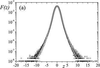
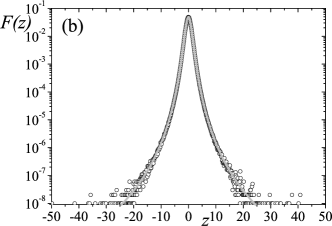
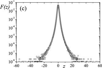
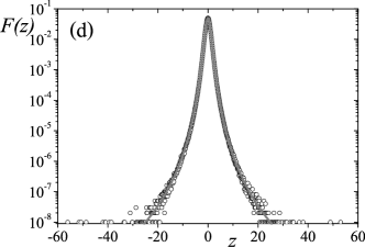
Figure 2: Typical runs of $ARCH\left(1\right)$ (Upper plots) and $GARCH\left(1,1\right)$ (Lower plots) with $\bar{\sigma}^{2}=1$. For each plot the symbols represent the relative frequency, $F\left(z\right)$, and the line the corresponding probability function, $\int_{z-\delta}^{z+\delta}p\left(\tilde{z}\right)\,d\tilde{z}$. In (a) $q=1.2424$ $\left(b=0.4;q_{n}=1\right)$; (b) $q=1.3464$ $\left(b=0.4;q_{n}=1.2\right)$; (c) $q=1.38$ $\left(b=0.4;c=0.4;q_{n}=1\right)$; (d) $q=1.35$ $\left(b=0.3;c=0.45;q_{n}=1.2\right)$.

By making the ansatz $P\left(z\right)$ $\simeq p\left(z\right)$, where $p\left(z\right)$ is the $q$-Gaussian probability density function which maximizes $S_{q}$ (Eq. (3)), and by imposing the matching of second ($\bar{\sigma}^{2}=1$) and fourth order moments, it is possible to establish, for $GARCH\left(1,1\right)$, a relation containing the dynamical parameters $b$ and $c$ and entropic indexes $q$ and $q_{n}$ :

$$b(5-3q_{n})(2-q)=\sqrt{(q-q_{n})-\left[(5-3\,q_{n})(2-q)-c^{2}(5-3\,q)(2-q_{n})\right]}-c(q-q_{n}).$$ (21)

For $c=0$, Eq. (21) reduces to the one corresponding to $ARCH\left(1\right)$,

$$q=\frac{q_{n}+2b^{2}\left(5-3q_{n}\right)}{1+b^{2}\left(5-3q_{n}\right)}$$ (22)

and, for $b=c=0$, one has $q=q_{n}$. The validity of Eqs. (21) and (22) is depicted in Fig. 2. The discrepancy between $p\left(z\right)$ and $P\left(z\right)$ can be evaluated by computing the sixth-order moment percentual difference, which is never greater than $3\%$ smdq-ct-arch ; smdq-ct-garch .

Since $\omega_{t}=z_{t}/\sigma_{t}$ and $\left\langle\omega_{t}\,\sigma_{t}\right\rangle=0$, for $q_{n}=1$ we can write

$$p\left(z|\sigma^{2}\right)=\frac{1}{\sqrt{2\,\pi\,\sigma^{2}}}\;e^{-\frac{z^{2}}{2\sigma^{2}}},$$

as the conditional probability density function of $z$ given $\sigma^{2}$. Considering that,

$$p\left(z\right)=\int\nolimits_{0}^{\infty}p\left(z|\sigma^{2}\right)\,P_{\sigma}\left(\sigma^{2}\right)\,d\left(\sigma^{2}\right),$$

and $P\left(z\right)$ $\simeq p\left(z\right)$, we obtain the stationary probability density function for squared volatilitysmdq-ct-garch ,

$$P_{\sigma}\left(\sigma^{2}\right)=\frac{\left(\sigma^{2}\right)^{-1-\lambda}}{\left(2\,\kappa\right)^{\lambda}\,\Gamma\left[\lambda\right]}\;e^{-\frac{1}{2\kappa\sigma^{2}}},$$

where

$$\lambda=\frac{1}{q-1}-\frac{1}{2},\qquad\kappa=\frac{1-q}{\bar{\sigma}^{2}\left(3q-5\right)}.$$

As one can observe in Fig. 3, the ansatz gives a quite satisfactory description for $\sigma^{2}$ probability density function, suggesting a connection between the $ARCH$ class of processes and nonextensive entropy. These explicit formulas can be helpful in applications related, among others, to option prices, where volatility forecasting plays a particularly important role.

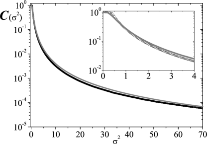
Figure 3: The symbols in black represent the inverse cumulative frequency, $C\left(\sigma^{2}\right)$, numerically obtained for a Gaussian noise with $b=c=0.4$ and the gray line the respective inverse cumulative distribution, $\int_{\sigma^{2}}^{\infty}P_{\sigma}\left(\tilde{\sigma}^{2}\right)\,d\left(\tilde{\sigma}^{2}\right)$ with $\left(\kappa,\lambda,\bar{\sigma}^{2}\right)=\left(0.444,2.125,1\right)$ for $P_{\sigma}\left(\tilde{\sigma}^{2}\right)$.

Albeit uncorrelated, stochastic variables $\left\{z_{t}\right\}$ are not independent. Applying the $q$-generalized Kullback-Leibler relative entropy tsallis-kl ; tsallis-borland-plastino to stationary joint probability density function $p_{1}\left(z_{t},z_{t-1}\right)$ and $p_{2}\left(z_{t},z_{t-1}\right)\equiv p\left(z_{t}\right)p\left(z_{t-1}\right)=$ $\left[p\left(z\right)\right]^{2}$ it is possible to quantify the degree of dependence between successive returns, through an optimal entropic index, $q^{op}$. In Ref. smdq-ct-garch , it was verified the existence of a direct relation between dependence, $q^{op}$, the non-Gaussianity, $q$, and the nature of the noise, $q_{n}$. An interesting property emerged, namely that, whatever be the pair $(b,c)$ that results in a certain $q$ for the stationary probability density function, one obtains the same $q^{op}$ and, consequently, the time series will present the same degree of dependence smdq-ct-garch . See Fig. 4.

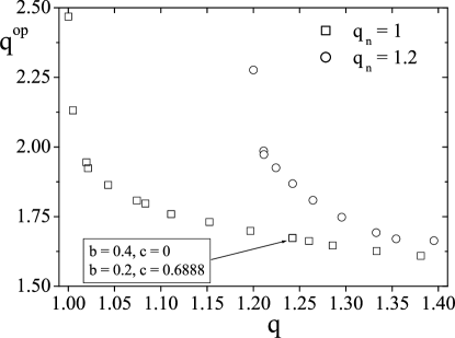
Figure 4: Plot of $q^{op}$ versus $q$ for typical $\left(b,c,q_{n}\right)$ triplets. The arrow points two examples which were obtained from different triplets and nevertheless coincide in what concerns the resulting point $\left(q,q^{op}\right)$.

It was also verified (see Fig. 5) for $ARCH\left(1\right)$ that the degree of dependence varies visibly with $b$ and with the lag $\tau$ between returns. This dependence would be related to a short-memory in volatility smdq-trends . The variance between these results and the empirical evidence of persistence in the real return time series dependence degree for time intervals up to $100$ days recently found, shows that financial markets dynamics are, in fact, ruled by some form of long-memory processes in volatility smdq-quantf .

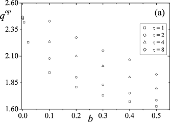
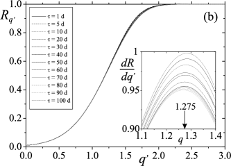
Figure 5: In panel (a) $q^{op}$ versus $b$ for $ARCH\left(1\right)$ process. Even for large allowed $b$ values, the decrease of dependence degree (i.e., increase of $q^{op}$) is visible when the time lag increases, which is not compatible with the empirical evidence of dependence degree around $q^{op}=1.275$ verified in Dow Jones return time series for time lags up to 100 days, panel (b). Comparing the two figures (a) and (b), it appears that financial markets present long-memory in the volatility similar to a $ARCH\left(n\right)$ process with $n\gg 1$.

Let us comment at this point that the connection between several entropic indexes, each one related to a different observable, is compatible with the dynamical scenario within which the nonextensive statistical mechanics is formulated. In fact, several entropic indexes emerge therein, coalescing onto the same value $q=1$ when ergodicity is verified.

IV.2 Mesoscopic models for traded volume in stock markets

Another important observable in financial markets is the traded volume $V$ (the number of shares of a stock traded in a period of time $T$). In Ref. osorio-borland-tsallis it was proposed an ansatz for the probability density function of high-frequency traded volume, which presents two power-law regimes (small and large values of $V$),

$$P\left(v\right)=\frac{1}{Z}\left(\frac{v}{{}^{\theta}}\right)^{\alpha}\exp_{q}\left(-\frac{v}{\theta}\right),$$ (23)

where $v$ represents the traded volume expressed in its mean value unit $\left\langle V\right\rangle$, i.e., $v=V/\langle V\rangle$, $\alpha$ and $\theta$ are positive parameters and $Z=\int_{0}^{\infty}(v/\theta)^{-\alpha}\exp_{q}\left(-\frac{v}{\theta}\right)dv$.

The probability density function (23) was recently obtained from a mesoscopic dynamical scenario smdq-vol based in the Feller process feller (using Itô definition),

$$dv=-\gamma\,\left(v-\frac{\alpha+1}{\beta}\right)\,dt+\sqrt{2\,v\,\frac{\gamma}{\beta}}\,dW_{t},$$ (24)

where instead of being constant in time, $\beta$ varies on a time scale much larger than the time scale of order $\gamma^{-1}$ needed to reach stationarity. The deterministic term of Eq. (24) represents a restoring market mechanism which tries to keep the traded volume in some typical value $\Theta=\frac{\alpha+1}{\beta}$ and the second term reflects stochastic memory and, basically, the effect of large traded volumes. In fact, large values of $v$ will provoke large amplitude of the stochastic term, leading to an increase or decrease of the traded volume (stirred or hush stock) depending on the sign of $W_{t}$. The fluctuation of $\beta$, alike to fluctuations in the mean value of $v$, can be related with changes in the activity volume due to agents herding mechanism caused by price movements or news.

Solving the corresponding Fokker-Planck equation for Eq. (24) we got the conditional probability of $v$ given $\beta$,

$$p\left(v|\beta\right)=\frac{\beta}{\Gamma\left[1+\alpha\right]}\left(\beta\,v\right)^{\alpha}\,\exp\left(-\beta\,v\right)\qquad(\alpha>-1,\ \beta>0).$$ (25)

Since

$$P\left(v\right)=\int_{0}^{\infty}P\left(v,\beta\right)\,\,d\beta=\int_{0}^{\infty}p\left(v|\beta\right)\,P\left(\beta\right)\,d\beta,$$ (26)

considering that $\beta$ follows a Gamma distribution,

$$P\left(\beta\right)=\frac{1}{\lambda\,\Gamma\left[\delta\right]}\left(\frac{\beta}{\lambda}\right)^{\delta-1}\exp\left(-\frac{\beta}{\lambda}\right)\qquad(\delta>0,\ \lambda>0),$$ (27)

Eq. (26) yields,

$$P\left(v\right)\equiv\frac{1}{Z}\left(\frac{v}{\theta}\right)^{\alpha}\exp_{q}\left(-\frac{v}{\theta}\right),$$ (28)

where, $q=1+1/(1+\alpha+\delta)$ and $\theta=(q-1)\lambda$. A numerical simulation for $1$ minute traded volume in NYSE stock index is exhibited in Fig. 6.

Figure 6: In panel (a) open symbols represents the PDF for the ten-high 1 minute traded volume stocks in NYSE exchange; solid symbols represent the PDF obtained for the numerical realization depicted in panel (b) and line the theoretical PDF Eq. (28). Parameters are $q=1.17$, $\alpha=1.79$, $\lambda=1.42$ and $\delta=3.09$.

Another possible mechanism to describe the dynamics of volumes, has been recently proposedadm on the basis of mean-reverting processes with additive-multiplicative structure, namely,

$$dv=-\gamma\,\left(v-\theta\right)\frac{1}{v}\,dt+\mu\sqrt{v}\,dW_{1}+\alpha dW_{2},$$ (29)

where, $\alpha$, $\mu$ are positive constants and $W_{1}$, $W_{2}$ independent standard Wienner processes. That is, following the ideas presented in Section III.1, in addition to fluctuations endogenously processed by the market, other fluctuations are taken into account that affect the dynamics directly. The stationary solution of the Fokker-Planck equation associated to the Itô-Langevin Eq. (29) has the form (28). Moreover, the underlying sequences present intermittent bursts (similar to those exhibited in Fig. 6.b) and, preliminary results indicate the presence of persistent power-law correlations, as observed in real data sequences.

Eq. (29) belongs to a larger class of processes with two-fold power-law behavior that can be also suitable for volumes, as well as, for other mean-reverting variables such as volatilities.

V Final remarks

Additive-multiplicative processes are at the core of nonextensive statistical mechanics. In the same natural way that standard Brownian motion leads to Gaussianity, linear additive-multiplicative stochastic processes lead to $q$-Gaussian distributions. Special (scale-invariant) correlations, that forbid convergence to the usual Gauss or Lévy limits, lead to a new type of statistical distributions. A remarkable feature is that the resulting power-law distributions may have exponents out of the Lévy range, thus allowing to embrace a larger variety of empirical processes. The presence of two Gaussian white noises, one either enhanced or reduced by internal information, and another purely exogenous, represents quite realistic features present in a variety of systems, thus justifying the ubiquity of the probability distributions associated to such kind of processes. In particular, as we have shown, they allow to model the dynamics of prizes, volatilities, stock-volumes and other relevant financial observables.

Another expression of the mechanism underlying the nonextensive theory is connected to the existence of a fluctuating intensive parameter (or “inverse temperature”) following the ideas that foundate the Beck and Cohen superstatistics beck-cohen . We have shown that these principles allow an alternative description of the dynamics of stock-volumes. Furthermore, such kind of mechanism allows an interesting perspective for treating the family of G/ARCH processes. The fact that the resulting probability density functions can be described in terms of $q$-Gaussian distributions, provides a tractable way of dealing with empirical distributions that match the G/ARCH types. Some of the discussions presented in this review have been done at a mesoscopic scale. The determination, from more microscopic models, of the parameters used at the mesoscopic scale is certainly welcome.

References

- (1) E. Fermi, Thermodynamics, (Doubleday, New York, 1936).
- (2) L. Boltzmann, Lectures on Gas Theory, (Dover, New York, 1995).
- (3) K. Huang, Statistical Mechanics, (John Wiley & Sons, New York, 1963).
- (4) A.I. Khinchin, Mathematical Foundations of Information Theory (Dover, New York, 1957) and Mathematical Foundations of Satistical Mechanics (Dover, New York, 1960).
- (5) B. Lesche, J. Stat. Phys. 27, 419 (1982)
- (6) V. Latora and M. Baranger, Phys. Rev. Lett. 273, 97 (1999).
- (7) C. Tsallis, J. Stat. Phys. 52, 479 (1988).
- (8) Curado E.M.F. and Tsallis C., J. Phys. A 24, L69 (1991); Corrigenda: 24, 3187 (1991) and 25, 1019 (1992); A 24, L69 (1991); Tsallis C., Mendes R. S. and Plastino A.R., Physica A 261, 534 (1998); see http://tsallis.cat.cbpf.br/biblio.htm for an updated bibliography.
- (9) C. Tsallis in Nonextensive Entropy - Interdisciplinary Applications, M. Gell-Mann and C. Tsallis (eds.) (Oxford University Press, New York, 2004).
- (10) C. Tsallis, Proceedings of the 31st Workshop of the International School of Solid State Physics “Complexity, Metastability and Nonextensivity”, held at the Ettore Majorana Foundation and Centre for Scientific Culture (Erice, July 2004), eds. C. Beck, A. Rapisarda and C. Tsallis (World Scientific, Singapore, 2005), in press [cond-mat/0409631]; Y. Sato and C. Tsallis, Proceedings of the Summer School and Conference on Complexity (Patras and Olympia, July 2004), ed. T. Bountis, International Journal of Bifurcation and Chaos (2005), in press [cond-mat/0411073]; C. Tsallis, M. Gell-Mann and Y. Sato, Special scale-invariant occupancy of phase space makes the entropy additive, [cond-mat/0502274] preprint, 2005.
- (11) Nonextensive Statistical Mechanics and its Applications, edited by S. Abe and Y. Okamoto, Lecture Notes in Physics Vol. 560 (Springer-Verlag, Heidelberg, 2001); Non-Extensive Thermodynamics and Physical Applications, edited by G. Kaniadakis, M. Lissia, and A. Rapisarda [Physica A 305 (2002)]; Anomalous Distributions, Nonlinear Dynamics and Nonextensivity, edited by H. L. Swinney and C. Tsallis [Physica D 193 (2004)]. Nonextensive Entropy - Interdisciplinary Applications, edited by M. Gell-Mann and C. Tsallis (Oxford University Press, New York, 2004).
- (12) Anteneodo C., Tsallis C., and Martinez A.S., Europhys. Lett. 59, 635 (2002).
- (13) C. Tsallis, C. Anteneodo, L. Borland and R. Osorio, Physica A 324, 89 (2003).
- (14) Kahneman D. and Tversky A., Econometrica 47, 263 (1979); Tversky A. and Kahneman D., Journal of Risk and Uncertainty 5, 297 (1992).
- (15) Gonzalez R. and Wu G., Cognitive Psychology 38, 129 (1999).
- (16) C. Tsallis, S.V.F Levy, A.M.C. de Souza and R. Maynard, Phys. Rev. Lett. 75, 3589 (1995); Erratum: ibid. 77, 5442 (1996).
- (17) S.M. Duarte Queirós, submitted to Quantitative Finance, 2004.
- (18) C. Anteneodo and C. Tsallis, J. Math. Phys. 44, 5194 (2003).
- (19) C. Anteneodo, preprint cond-mat/0409035.
- (20) H. Sakaguchi, J. Phys. Soc. Jpn. 70, 3247 (2001).
- (21) G. Kaniadakis and P. Quarati, Physica A 237, 229 (1997).
- (22) L. Borland, Phys. Rev. Lett 89, 098701 (2002).
- (23) A.R. Plastino, A. Plastino, Physica A 222, 347 (1995); C. Tsallis, D.J. Bukman, Phys. Rev. E 54 R2197 (1996).
- (24) S.L. Heston. Rev. Fin. Stud. 6, 327 (1993).
- (25) G. Wilk and Z. Włodarczyk, Phys. Rev. Lett. 84, 2770 (2000).
- (26) C. Beck and E.G.D. Cohen, Physica A 322, 267 (2003).
- (27) B.B. Mandelbrot, J. Bus. 36, 394 (1963); E.F. Fama, J. Bus. 38, 34 (1965).
- (28) A. Lo, Econometrica 59, 1279 (191); Z. Ding, C.W.J. Granger amd R.F. Engle, J. Empirical Finance 1, 83 (1993).
- (29) R.F. Engle, Econometrica 50, 987 (1982).
- (30) J. Hull and A. White, J. Fin. 42, 281 (1987); E.M. Stein and J.C. Stein, Rev. Fin. Stud. 4, 727 (1991); M. Potters, R. Cont and J.-P. Bouchaud, Europhys. Lett. 41, 239 (1998).
- (31) J.P. Fouque, G. Papanicolaou and K.R. Sircar, Derivatives in Financial Markets with Stochastic Volatility, (Cambridge University Press, Cambridge) 2000.
- (32) T. Bollerslev, R.Y. Chou and K.F. Kroner, J. of Econometrics 52, 5 (1992).
- (33) P. Embrechts, C. Kluppelberg and T. Mikosch, Modelling Extremal Events for Insurance and Finance (Applications of Mathematics), (Springer-Verlag, Berlin) 1997.
- (34) T. Bollerslev, J. of Econometrics 31, 307 (1986).
- (35) E. Scalas, R. Gorenflo and R. Mainardi, Physica A 284, 367 (2000).
- (36) R.F. Engle and J. Russel, Econometrica 66, 1127 (1998).
- (37) S.M. Duarte Queirós and C. Tsallis, Europhys. Lett. (in press, 2005), preprint avaible at cond-mat/0401181.
- (38) S.M. Duarte Queirós and C. Tsallis, preprint cond-mat/0502151.
- (39) C. Tsallis, Phys. Rev. E 58, 1442 (1998).
- (40) L. Borland, A.R. Plastino and C. Tsallis, J. Math. Phys. 39, 6490 (1998) [Erratum: J. Math. Phys. 40, 2196 (1999)].
- (41) S.M. Duarte Queirós, Physica A 344, 619 (2004).
- (42) R. Osorio, L. Borland and C. Tsallis in Nonextensive Entropy - Interdisciplinary Applications, M. Gell-Mann and C. Tsallis (eds.) (Oxford University Press, New York, 2004).
- (43) S.M. Duarte Queirós, preprint cond-mat/0502337.
- (44) W. Feller, Ann. of Math. 54, 173 (1951).
- (45) C. Anteneodo and R. Riera, preprint physics/0502119.