Scaling laws for the movement of people between locations in a large city

Abstract

Large scale simulations of the movements of people in a “virtual” city and their analyses are used to generate new insights into understanding the dynamic processes that depend on the interactions between people. Models, based on these interactions, can be used in optimizing traffic flow, slowing the spread of infectious diseases or predicting the change in cell phone usage in a disaster. We analyzed cumulative and aggregated data generated from the simulated movements of $1.6$ million individuals in a computer (pseudo agent-based) model during a typical day in Portland, Oregon. This city is mapped into a graph with $181,206$ nodes representing physical locations such as buildings. Connecting edges model individual’s flow between nodes. Edge weights are constructed from the daily traffic of individuals moving between locations. The number of edges leaving a node (out-degree), the edge weights (out-traffic), and the edge-weights per location (total out-traffic) are fitted well by power law distributions. The power law distributions also fit subgraphs based on work, school, and social/recreational activities. The resulting weighted graph is a “small world” and has scaling laws consistent with an underlying hierarchical structure. We also explore the time evolution of the largest connected component and the distribution of the component sizes. We observe a strong linear correlation between the out-degree and total out-traffic distributions and significant levels of clustering. We discuss how these network features can be used to characterize social networks and their relationship to dynamic processes.

1 Introduction

Similar scaling laws and patterns have been detected in a great number of systems found in nature, society, and technology. Networks of scientific collaboration [1][2][3], movie actors [4], cellular networks [5][6], food webs [7], the Internet [8], the World Wide Web [9, 10], friendship networks [11] and networks of sexual relationships [12] among others have been analyzed up to some extent. Several common properties have been identified in such systems. One such property is the short average distance between nodes, that is, a small number of edges need to be traversed in order to reach a node from any other node. Another common property is high levels of clustering [4, 13], a characteristic absent in random networks [14]. Clustering measures the probability that the neighbors of a node are also neighbors of each other. Networks with short average distance between nodes and high levels of clustering have been dubbed “small worlds” [4, 13]. Power-law behavior in the degree distribution is another common property in many real world networks [15]. That is, the probability that a randomly chosen node has degree $k$ decays as $P(k)\sim k^{-\gamma}$ with $\gamma$ typically between $2$ and $3$. Barabási and Albert (BA) introduced an algorithm capable of generating networks with a power-law connectivity distribution ($\gamma=3$). The BA algorithm generates networks where nodes connect, with higher probability, to nodes that have a accumulated higher number of connections and stochastically generates networks with a power-law connectivity distributions in the appropriate scale.

Social networks are often difficult to characterize because of the different perceptions of what a link constitutes in the social context and the lack of data for large social networks of more than a few thousand individuals. Even though detailed data on the daily movement of people in a large city does not exist, these systems have been statistically sampled and the data used to build detailed simulations for the full population. The insights gained by studying the simulated movement of people in a virtual city can help guide research in identifying what scaling laws or underlying structures may exist and should be looked for in a real city. In this article we analyze a social mobility network that can be defined accurately by the simulated movement of people between locations in a large city. We analyze the cumulative directed graph generated from the simulated movement of $1.6$ million individuals in or out of $181,206$ locations during a typical day in Portland, OR. The $181,206$ nodes represent locations in the city and the edges connections between nodes. The edges are weighted by daily traffic (movement of individuals) in or out of these locations. The statistical analysis of the cumulative network reveals that it is a small world with power-law decay in the out-degree distribution of locations (nodes). The resulting graph as well as subgraphs based on different activity types exhibit scaling laws consistent with an underlying hierarhical structure [16, 17]. The out-traffic (weight of the full network) and the total out-traffic (total weight of the out edges per node) distributions are also fitted to power laws. We show that the joint distribution of the out-degree and total out-traffic distributions decays linearly in an appropriate scale. We also explore the time evolution of the largest component and the distribution of the component sizes.

1.1 Transportation Analysis Simulation System (TRANSIMS)

TRANSIMS [18] is an agent-based simulation model of the daily movement of individuals in virtual region or city with a complete representation of the population at the level of households and individual travelers, daily activities of the individuals, and the transportation infrastructure. The individuals are endowed with demographic characteristics taken from census data and the households are geographically distributed according to the population distribution. The transportation network is a precise representation of the city’s transportation infrastructure. Individuals move across the transportation network using multiple modes including car, transit, truck, bike, walk, on a second-by-second basis. DMV records are used to assign vehicles to the households so that the resulting distribution of vehicle types matches the actual distribution. Individual travelers are assigned a list of activities for the day (including home, work, school, social/recreational, and shop activities) obtained from the household travel activities survey for the metropolitan area [19] (Figure 2 shows the frequency of four activity types in a typical day). Data on activities also include origins, destinations, routes, timing, and forms of transportation used. Activities for itinerant travelers such as bus drivers are generated from real origin/destination tables.
TRANSIMS consists of six major integrated modules: Population synthesizer, Activity Generator, Router, Microsimulation and Emissions Estimator. Detailed information on each of the modules is available [18]. TRANISMS has been designed to give transportation planners accurate, complete information on traffic impacts, congestion, and pollution.

For the case of the city of Portland, OR, TRANSIMS calculates the simulated movements of 1.6 million individuals in a typical day. The simulated Portland data set includes the time at which each individual leaves a location and the time of arrival to its next destination (node). These data are used to calculate the average number of people at each location and the traffic between any two locations on a typical day. (Table $1$ shows a sample of a Portland activity file generated by TRANSIMS). Locations where activities are carried out are estimated from observed land use patterns, travel times and costs of transportation alternatives. These locations are fed into a routing algorithm that finds the minimum cost paths that are consistent with individual choices [20, 21, 22]. The simulation land resolution is of 7.5 meters. The simulator provides an updated estimate of time-dependent travel times for each edge in the network, including the effects of congestion, to the Router and location estimation algorithms [18], which generate traveling plans. Since the entire process estimates the demand on a transportation network from census data, land use data, and activity surveys, these estimates can thus be applied to assess the effects of hypothetical changes such as building new infrastructures or changing downtown parking prices. Methods based on observed demand cannot handle such situations, since they have no information on what generates the demand. Simulated traffic patterns compare well to observed traffic and, consequently, TRANSIMS provides a useful planning tool.

Until recently, it has been difficult to obtain useful estimates on the structure of social networks. Certain classes of random graphs (scale-free networks [15], small-world networks [11, 13], or Erdos-Renyi random graphs [14, 23]), have been postulated as good representatives. In addition, data based models while useful are limited since they have naturally focused on small scales [24]. While most studies on the analysis of real networks are based on a single snapshot of the system, TRANSIMS provides powerful time dependent data of the evolution of a location-based network.

2 Portland’s location-based network

A “typical” realization by the Transportation Analysis Simulation System (TRANSIMS) simulates the dynamics of $1.6$ million individuals in the city of Portland as a directed network, where the nodes represent locations (i.e. buildings, households, schools, etc.) and the directed edges (between the nodes) represent the movement (traffic due to activities) of individuals between locations (nodes). We have analyzed the cumulative network of the whole day as well as cumulative networks that comprise different time intervals of the day. Here we use the term “activity” to denote the movement of an individual to the location where the activity will be carried out. Traffic intensity is modeled by the nonsymmetric mobility matrix $W=(w_{ij})$ of traffic weights assigned to all directed edges in the network ($w_{ij}=0$ means that there is no directed edge connecting node $i$ to node $j$).

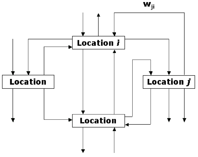
Figure 1: Structure of the location-based network of the city of Portland. The nodes represent locations connected via directed edges based on the traffic or movement of individuals (activities) between the locations. The weights ($w_{ij}$) of the edges represent the daily traffic from location $i$ to location $j$.

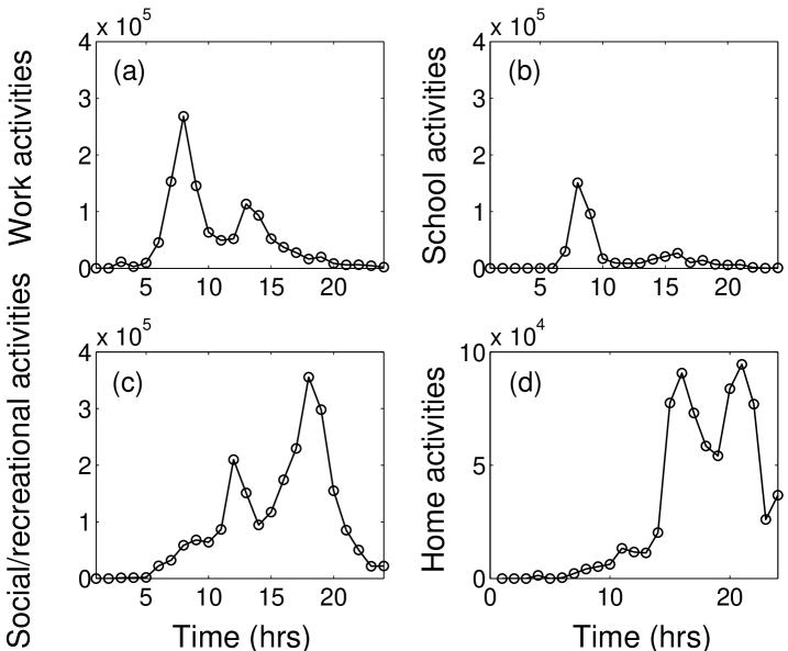
Figure 2: The number of people active in (a) work activities, (b) school activities, (d) social activities, and (d) home activities as a function of time (hours) during a ‘typical’ day in Portland, Oregon.

Person ID	Location ID	Arrival time(hrs)	Departure time(hrs)	Activity type
115	4225	0.0000	7.00	home
115	49296	8.00	11.00	work
115	21677	11.2	13.00	work
115	49296	13.2	17.00	work
115	4225	18.00	19.00	home
115	33005	19.25	21.00	social/rec
115	4225	21.3	7.00	home
220	8200	0.0000	8.50	home
220	10917	9.00	14.00	school
220	8200	14.5	18.00	home
220	3480	18.2	20.00	social/rec
220	8200	20.3	8.6	home

Table 1: Sample section of a TRANSIMS activity file. In this example, person $115$ arrives for a social recreational activity at location $33005$ at $19.25$ o’clock and departs at $21.00$ o’clock.

3 Power law distributions

We calculate the statistical properties of a typical day in the location-based network of this vitual city from the cumulative mobility data generated by TRANSIMS (see Table 2).
The average out-degree is $<k>=\sum^{n}_{i=1}k_{i}/n$ where $k_{i}$ is the degree for node $i$ and $n$ is the total number of nodes in the network. For the portland network $<k>=29.88$ and the out-degree distribution exhibits power law decay with scaling exponent ($\gamma\approx 2.7$). The out-traffic (edge weights) and the total out-traffic (edge-weights per node) distributions are also fitted well by power laws.

The average distance between nodes $L$ is defined as the median of the means $L_{i}$ of the shortest path lengths connecting a vertex $i\in V(G)$ to all other vertices [25]. For our network, $L=3.1$, which is small when compared to the size of the network. In fact, the diameter ($D$) of the graph (the largest of all possible shortest paths between all the locations) is only $8$. $L$ and $D$ are measured using a breadth first search (BFS) algorithm [26] ignoring the edge directions.

The clustering coefficient, $C$, quantifies the extent to which neighbors of a node are also neighbors of each other [25]. The clustering coefficient of node $i$, $C_{i}$, is given by

$$C_{i}=\left|E(\Gamma_{i})\right|/\binom{k_{i}}{2}$$

where $\left|E(\Gamma_{i})\right|$ is the number of edges in the neighborhood of $i$ (edges connecting the neighbors of $i$ not including $i$ itself) and $\binom{k_{i}}{2}$ is the maximal number of edges that could be drawn among the $k_{i}$ neighbors of node $i$. The clustering coefficient $C$ of the whole network is $C=\sum^{n}_{i=1}C_{i}/n$. For a scale-free random graph (BA model) [15] with $181,206$ nodes and $m=16$ [27], the clustering coefficient $C_{rand}\approx\frac{(m-1)}{8}\frac{(lnN)^{2}}{N}\approx 0.0015$ [28, 29]. The clustering coefficient for our location-based network, ignoring edge directions, is $C=0.0584$, which is roughly $39$ times larger than $C_{rand}$.

Highly clustered networks have been observed in other systems [4] including the electric power grid of western US. This grid has a clustering coefficient $C=0.08$, about 160 times larger than the expected value for an equivalent random graph [25]. The few degrees of separation between the locations of the (highly clustered) network of the city of Portland “make” it a small world [13, 11, 25].

Statistical properties	Value
Total nodes ($N$)	181,206
Size of the cumulative largest component ($S$)	181,192
Total directed edges ($E$)	5,416,005
Average out-degree ($<k>$)	29.88
Clustering coefficient ($C$)	0.0584
Average distance between nodes ($L$)	3.1
Diameter ($D$)	8.0

Table 2: Statistical properties of the Portland’s location-based network. $S$ is the size of the largest component of the cumulative network during the whole day.

Many real-world networks exhibit properties that are consistent with underlying hierarhical organizations. These networks have groups of nodes that are highly interconnected with few or no edges connected to nodes outside their group. Hierarchical structures of this type have been characterized by the clustering coefficient function $C(k)$, where $k$ is the node degree. A network of movie actors, the semantic web, the World Wide Web, the Internet (autonomous system level), and some metabolic networks [16, 17] have clustering coefficients that scale as $k^{-1}$. The clustering coefficient as a function of degree (ignoring edge directions) in the Portland network exhibits similar scaling at various levels of aggregation that include, the whole network and subnetworks constructed by activity type (work, school and social/recreational activities, see Figure 3). We constructed subgraphs based on activity types, that is, those subgraphs constructed from all the directed edges of a specific activity type (i.e work, school, social) during a typical day in the city of Portland. The clustering coefficient of the subnetworks generated from work, school, and social/recreational activities are: $0.0571$, $0.0557$, and $0.0575$, respectively. The largest clustering coefficient and closest to the overall clustering coefficient ($C=0.0584$) correponds to the subnetwork constructed from social/recreational activities. It seems that the whole network, as well as the selected activity subnetworks, support a hierarchical structure albeit the nature of such structure (if we choose to characterize by the power law exponent) is not universal. This agrees with relevant theory [17].

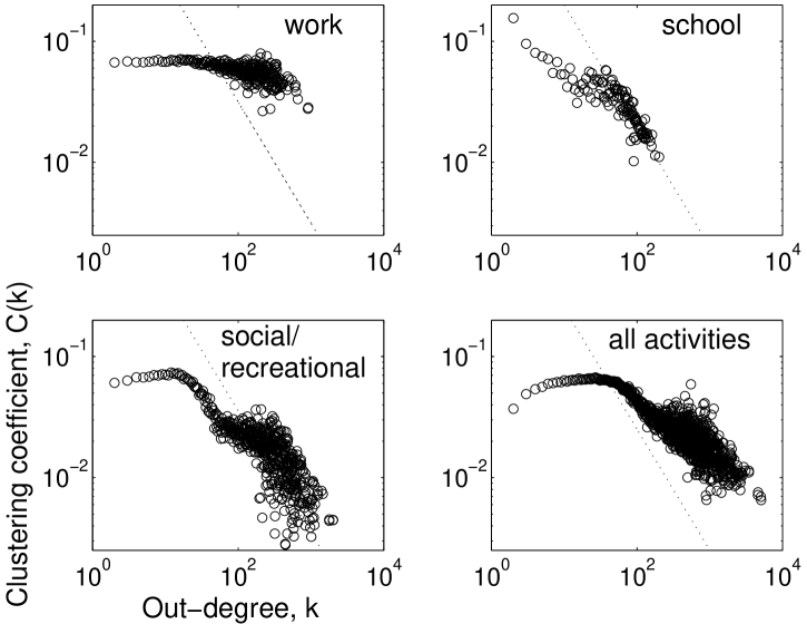
Figure 3: Log-log plots of the clustering coefficient as a function of the out-degree for subnetworks constructed from work activities, school activities, social activities, and all the activities. The dotted line has slope $-1$. Notice the scaling $k^{-1}$ for the school and social/recreational activities. However, for the subnetwork constructed from work activities, the clustering coefficient is almost independent of the out-degree $k$.

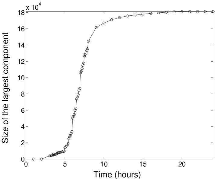
Figure 4: The size of the largest component (cluster) over time. A sharp transition is observed at about 6 a.m when people move from home to work or school.

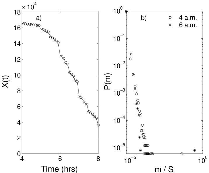
Figure 5: (a) The number of components $X(t)$ between $4$ a.m. and $8$ a.m. (b) Probability distribution $P(m)$ of the normalized component sizes at two different times of the day. The component sizes ($m$) have been normalized by $S$, the size of the largest component of the cumulative network during the whole day (Table $1$).

Time (hrs)	Size of largest component
5.6	27,132
5.8	31,511
6.0	50,242
6.2	54,670
6.4	62,346
6.6	76,290
6.8	84,516
7.0	106,160

Table 3: Size of the largest component just before and after 6 a.m., the time at which a sharp transition occurs. At midnight, all but 14 locations belong to the largest component (Table $2$).

Understanding the temporal properties of networks is critical to the study of superimposed dynamics such as the spread of epidemics on networks. Most studies of superimposed processes on networks assumes that the contact structure is fixed (see for example [30, 31, 32, 33, 34, 35, 36, 37, 38]). Here, we take a look at the time evolution of the largest connected component of the location-based network of the city of Portland (Figure 4). We have observed that a sharp transition occurs at about $6$ a.m. In fact, by $7$ a.m. the size of the largest component includes approximately $60\%$ of the locations (nodes). Table $3$ shows the size of the largest component just before and after the sharp transition occurs.

Let $X_{m}(t)$ be the number of components of size $m$ at time $t$. Then $X(t)=\sum_{m\geq 1}X_{m}(t)$ is the total number of components at time t (Figure 5(a)). Furthermore, the probability $P(m)$ that a randomly chosen node (location) belongs to a component of size $m$ follows a power law that gets steeper in time as the giant component forms (Figure 5(b)).

To identify the relevance of the temporal trends, we computed the out-degree distribution of the network for three different time intervals: The morning from $6$ a.m to $12$ p.m.; the workday from $6$ a.m. to 6 p.m.; and the full $24$ hours. In the morning phase, the out-degree distribution has a tail that decays as a power law with $\gamma\simeq 2.7$ (for the workday $\gamma\simeq 2.43$ and for the full day $\gamma\simeq 2.4$). The distribution of the out-degree data has two scaling regions: the number of locations is approximately constant for out-degree $k<20$ and then decays as a power law for high degree nodes (Fig. 6). The degree distribution for the undirected network (ignoring edge direction) displays power-law behavior, but with slightly different power-law exponents: $2.3$ (morning), $2.48$ (work day) and $2.51$ (full day).

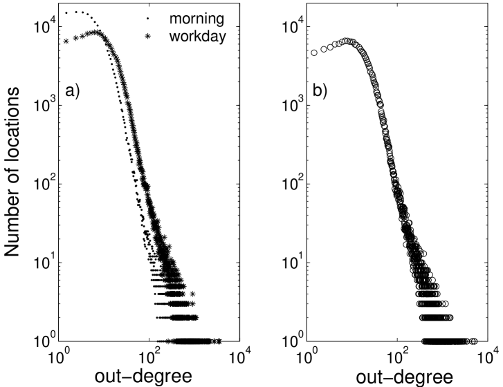
Figure 6: Distribution of the out-degrees of the location-based network of the city of Portland. There are approximately the same number of nodes (locations) with out-degree $k=1,2,...10$. For $k>10$ the number of nodes with a given out-degree decays as a power law $P(k)\propto k^{-\gamma}$ with (a) $\gamma\simeq 2.7$ for the morning (6 a.m.-12 p.m.), $\gamma\simeq 2.43$ for the workday (6 a.m.-6 p.m.) and (b) $\gamma\simeq 2.4$ for the full day.

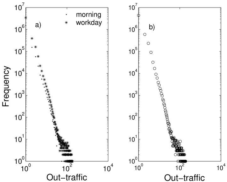
Figure 7: The out-traffic distribution of the location-based network of the city of Portland follows a power law ($P(k)\propto k^{-\gamma}$) with (a) $\gamma\approx 3.56$ (morning), $\gamma\approx 3.74$ (afternoon), and (b) $\gamma\approx 3.76$ (full day). Hence a few connections have high traffic but most connections have low traffic.

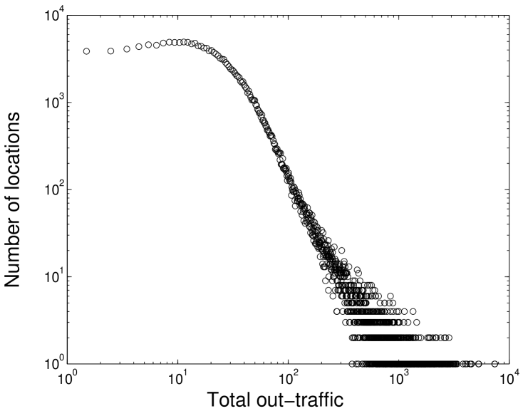
Figure 8: Distribution of the total out-traffic for the location-based network of the city of Portland. There are approximately the same number of locations (nodes) with small total out-traffic. The number of locations where more than 30 people (approximately) leave each day decays as a power law with $\gamma\simeq 2.74$.

The strength of the connections in the location-based network is measured by the traffic (flow of individuals) between locations in a “typical” day of the city of Portland. The log-log plot of the out-traffic distributions for three different periods of time (Fig. 7) exhibits power law decay with exponents, $\gamma\simeq 3.56$ for the morning, $\gamma\simeq 3.74$ for the workday, and $\gamma\simeq 3.76$ for the full day. The out-traffic distribution is characterized by a power law distribution for all values of the traffic-weight matrix $W$. This is not the case for the out-degree distribution of the network (see Figure 6) where a power law fits well only for sufficiently large degree $k$ ($k>10)$.
The distribution of the total out-traffic per location, $w_{i}$’s ($w_{i}=\sum_{j}w_{i,j}$), is characterized by two scaling regions. The tail of this distribution decays as a power law with exponent $\gamma=2.74$ (Fig. 8). This is almost the same decay as the out-degree distribution ($\gamma=2.7$) because the out-degree and the total out-traffic are highly correlated (with correlation coefficient $\rho=0.94$).

4 Correlation between out-degree and total out-traffic

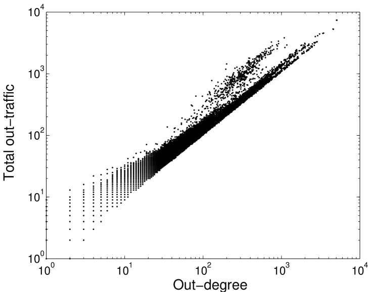
Figure 9: Correlation between the out-degree and the total out-traffic. The correlation coefficient is $\rho=0.94$ on a log-log scale. Most ($95\%$) of the locations have fewer than $100$ people leaving during the day.

The degree of correlation between various network properties depend on the social dynamics of the population. The systematic generation and resulting structure of these networks is important to understand dynamic processes such as epidemics that “move” on these networks. Understanding the mechanisms behind these correlations will be useful in modeling fidelity networks.

In the Portland network, the out-degree $k$ and total out-traffic $v$ have a correlation coefficient $\rho=0.94$ on a log-log scale with $95\%$ of the nodes (locations) having out-degree and total out-traffic less than $100$ (Fig. 9). That is, the density of their joint distribution $F(k,v)$ is highly concentrated near small values of the out-degree and total out-traffic distributions. The joint distribution supports a surface that decays linearly when the density is in $log_{e}$ scale (Figure LABEL:myfig5).

5 Conclusions

Strikingly similar patterns on data from the movement of $1.6$ million individuals in a “typical” day in the city of Portland have been identified at multiple temporal scales and various levels of aggregation. The analysis is based on the mapping of people’s movement on a weighted directed graph where nodes correspond to physical locations and where directed edges, connecting the nodes, are weighted by the number of people moving in and out of the locations during a typical day. The clustering coefficient, measuring the local connectedness of the graph, scales as $k^{-1}$ ($k$ is the degree of the node) for sufficiently large $k$. This scaling is consistent with that obtained from models that postulate underlying hierarhical structures (few nodes get most of the action). The out-degree distribution in log-log scale is relatively constant for small $k$ but exhibits power law decay afterwards ($P(k)\propto k^{-\gamma}$). The distribution of daily total out-traffic between nodes in log-log scale is flat for small $k$ but exhibits power law decay afterwards. The distribution of the daily out-traffic of individuals between nodes scales as a power law for all $k$ (degree).
The observed power law distribution in the out-traffic (edge weights) is therefore, supportive of the theoretical analysis of Yook et al. [39] who built weighted scale-free (WSF) dynamic networks and proved that the distribution of the total weight per node (total out-traffic in our network) is a power law where the weights are exponentially distributed.
There have been limited attempts to identify at least some characteristics of the joint distributions of network properties. The fact that daily out-degree and total out-traffic data are highly correlated is consistent again with the results obtained from models that assume an underlying hierarhical structure (few nodes have most of the connections and get most of the traffic (weight)). The Portland network exhibits a strong linear correlation between out-degree and total out-traffic on a log-log scale. We use this time series data to look at the network “dynamics”. As the activity in the network increases, the size of the maximal connected component exhibits threshold behavior, that is, a “giant” connected component, suddenly emerges. The study of superimposed processes on networks such as those associated with the potential deliberate release of biological agents needs to take into account the fact that traffic is not constant. Planning, for example, for worst-case scenarios requires knowledge of edge-traffic, in order to characterize the temporal dynamics of the largest connected network components [40].

6 Acknowledgements

The authors thank Pieter Swart, Leon Arriola, and Albert-László Barabási for interesting and helpful discussions. This research was supported by the Department of Energy under contracts W-7405-ENG-36 and the National Infrastructure Simulation and Analysis Center (NISAC).

References

- [1] M.E.J. Newman, Proc. Natl. Acad. Sci. USA 98, 404-409 (2001).
- [2] M. E. J. Newman, Phys. Rev. E 64 016131 (2001); Phys. Rev. E 64 016132 (2001).
- [3] A.-L. Barabási, H. Jeong, R. Ravasz, Z. Néda, T. Vicsek, and A. Schubert, Physica A 311, 590-614 (2002).
- [4] D. J. Watts and S. H. Strogatz, Nature 363, 202-204 (1998).
- [5] H. Jeong, B. Tombor, R. Albert, Z.N. Oltvai, and A.-L. Barabási, Nature 407, 651-654 (2000).
- [6] H. Jeong, S. Mason, A.-L. Barabási, and Z.-N. Oltvai, Nature 411, 41-42 (2001).
- [7] R.J. Williams, E.L. Berlow, J.A. Dunne, A.-L. Barabási, and N.D. Martinez. Two degrees of separation in complex food webs, Proc. Natl. Acad. Sci. USA 99, 12913-12916 (2002).
- [8] M. Faloutsos, P. Faloutsos, C. Faloutsos, On Power-Law Relationships of the Internet topology, SGCOMM (1999).
- [9] R. Albert, H. Jeong, and A.-L. Barabási, Nature 401, 130-131 (1999).
- [10] R. Kumar, P. Raghavan, S. Rajagopalan, D. Sivakumar, A.S. Tomkins, E. UpfalProc, 19th ACM SIGACT-SIGMOD-AIGART Symp. Principles of Database Systems, PODS (2000).
- [11] L. A. N. Amaral, A. Scala, M. Barthelemy, and H. E. Stanley, Proc. Natl. Acad. Sci. 97(21), 11149-52. (2000).
- [12] F. Liljeros, C. R. Edling, L. A. Nunes Amaral, H. E. Stanley, Y. berg, The Web of Human Sexual Contacts, Nature 411, 907-908 (2001).
- [13] S.H. Strogatz, Exploring Complex Networks, Nature 410, 268-276 (2001).
- [14] B. Bollobás, Random Graphs, Academic, London (1985).
- [15] Albert-László Barabási, Réka Albert, Hawoong Jeong, Physica A 272, 173-87 (1999).
- [16] E. Ravasz, A. L. Somera, D. A. Mongru, Z. N. Oltvai,and A.-L. Barabási, Science 297, 1551-1555 (2002).
- [17] Erzsébet Ravasz and A.-L. Barabási, Phys. Rev. E 67, 026112 (2003).
- [18] C.L. Barret et al. TRANSIMS: Transportation Analysis Simulation System. LA-UR-00-1725, Los Alamos National Laboratory Unclassified Report LA-UR-00-1725 (2001). TRANSIMS website: http://www-transims.tsasa.lanl.gov/
- [19] National Household Travel Survey (NHTS). Website: http://www.dmampo.org/313.html
- [20] C. Barrett, K. Bisset, R. Jacob, G. Konjevod, and M. Marathe. An Experimental Analysis of a Routing Algorithm for Realistic Transportation Networks. to appear in European Symposium on Algorithms (ESA). Los Alamos Unclassified Report LA-UR-02-2427 (2002).
- [21] C. Barrett, R. Jacob, and M. Marathe. Formal Language Constrained Path Problems. SIAM J. Computing, 30(3):809–837 (2001).
- [22] R. Jacob, M. Marathe, and K. Nagel. A Computational Study of Routing Algorithms for Realistic Transportation Networks. ACM J. Experimental Algorithmics, 4:6, 1999. http://www.jea.acm.org/1999/JacobRouting/.
- [23] P. Erdos and A. Renyi. On the evolution of random graphs. Publications of the Mathematical Institute of the Hungarian Academy of Sciences, 5:17-61 (1960).
- [24] D. Peterson, L. Gatewood, Z. Zhuo, J. J. Yang, S. Seaholm, and E. Ackerman. Simulation of stochastic micropopulation models. Computers in Biology and Medicine, 23(3):199-210 (1993).
- [25] D. J. Watts, Small Worlds: The dynamics of networks between order and randomness, Princeton University Press (1999).
- [26] R. Sedgewick, Algorithms, Addison-Wesley (1988).
- [27] is constant for the BA model. We have used , the median out-degree of our network.
- [28] K. Klemm, V.M. Eguiluz, Phys. Rev. E 65, 057102 (2002).
- [29] A. Fronczak, P. Fronczak, J. A. Holyst, cond-mat/0306255.
- [30] P. Grassberger, Math. Biosc. 63, 157-172 (1983).
- [31] M. E. J. Newman, Phys. Rev. E 66 016128 (2002).
- [32] M. E. J. Newman, I. Jensen, and R. M. Ziff, Phys. Rev. E 65 021904 (2002).
- [33] C. Moore and M. E. J. Newman, Phys. Rev. E 61, 5678-5682 (2000).
- [34] R. Pastor-Satorras and A. Vespignani, Phys. Rev. E 63, 066117 (2001).
- [35] R. Pastor-Satorras and A. Vespignani, Phys. Rev. E 65 036104 (2002).
- [36] R. M. May and A. L. Lloyd, Phys. Rev. E 64, 066112 (2001).
- [37] Z. Dezso and A.-L. Barabási, Phys. Rev. E 65, 055103 (2002).
- [38] V. M. Eguíluz and K. Klemm, Phys. Rev. Lett. 89, 108701 (2002).
- [39] S.H. Yook, H. Jeong, A.-L. Barabási and Y. Tu, Physical Rev. Lett. 86, 5835 (2001).
- [40] G. Chowell and C. Castillo-Chavez, Worst-Case Scenarios and Epidemics, in Mathematical and Modeling Approaches in Homeland Security. SIAM’s series Frontiers in Applied Mathematics (September, 2003).