Why does the Standard GARCH(1,1) model work well?

Abstract

The AutoRegressive Conditional Heteroskedasticity (ARCH) and its generalized version (GARCH) family of models have grown to encompass a wide range of specifications, each of them is designed to enhance the ability of the model to capture the characteristics of stochastic data, such as financial time series. The existing literature provides little guidance on how to select optimal parameters, which are critical in efficiency of the model, among the infinite range of available parameters. We introduce a new criterion to find suitable parameters in GARCH models by using Markov length, which is the minimum time interval over which the data can be considered as constituting a Markov process. This criterion is applied to various time series and results support the known idea that GARCH(1,1) model works well.

I Introduction

The ARCH model Engle1 and standard GARCH model Bollerslev1 are now not only widely used in the Foreign Exchange (FX) literature Bollerslev2 but also as the basic framework for empirical studies of the market micro-structure such as the impact of news Goodhart1 and government interventions Goodhart2 ; Peiers , or inter- and intra-market relationships Engle2 ; Baillie . Due to basic similarities between the mentioned models of different constants, here we focus our discussion on financial context.

The main assumption behind this class of models is the relative homogeneity of the price discovery process among market participants at the origin of the volatility process. Volatility is an essential ingredient for many applied issues in finance. It is becoming more important to have a good measure and forecast of short-term volatility, mainly at the one to ten day horizon. Currently, the main approaches to compute volatilities are by historical indicators computed from daily squared or absolute valued returns, by econometric models such as GARCH. In other words, the conditional density of one GARCH process can adequately capture the information. In particular, GARCH parameters for the weekly frequency theoretically derived from daily empirical estimates are usually within the confidence interval of weekly empirical estimates Drost . It is interesting to note that despite the extensive list of models which now belong to the ARCH family Andersen ; Bera ; Bollerslev3 , the existing literature provides little guidance on how to select optimal $q$ and $p$ values in a GARCH ($q$,$p$) model. The two parameters $q$ and $p$ in GARCH model refer to history of the return and volatility of time series, respectively. However, there are some criteria to find the suitable $q$ and $p$. Pagan and Sabu Pagan , suggest a misspecified volatility equation that can result in inconsistent maximum likelihood estimates of the conditional mean parameters Solibakke . Further West and Cho West show how appropriate GARCH model selection can be used to enhance the accuracy of exchange rate volatility forecasts. However, there is an almost ubiquitous reliance on the standard GARCH (1,1)-type model in the applied literature. In this paper, we suggest a new approach to find optimal values $q$ and $p$. In our approach, a fundamental time scale is the Markov time scale, $t_{M}$, which is the minimum time interval over which the data can be considered as constituting a Markov process. As our starting point, we proceed by stressing on the role of $q$ and $p$ in the GARCH model and their similarity to the Markov length scale in stochastic processes. There are reported examples of measuring Markov length for various data Friedrich1 ; Siefert . Recently Tabar et al., Bhattacharyya , have used the dynamics of the Markov length for predicting earthquakes. Moreover, Renner et al. Renner have shown that Markov time scale in returns of the high frequency (minutely) US Dollar - German Mark exchange rates in the one-year period October 92 to September 93 is larger than 4 minutes.

Generally, we check whether the data follow a Markov chain and, if so, measure the Markov length scale, $t_{M}$. Such a given process with a degree of randomness or stochasticity may have a finite or an infinite Markov length scale. Specifically, the Markov length scale is the minimum length interval over which the data can be considered as a Markov process. The main goal of this paper is to utilize the mentioned similarity between the role of $q$ and $p$ in the GARCH model and Markov time scale in stochastic processes, and introduce a novel method to estimate optimal GARCH model parameters of daily data.

II GARCH Based Volatility Models

The GARCH model, which stand for Generalized AutoRegressive Conditional Heteroscedasticity, is designed to provide a volatility measure like a standard deviation that can be used in financial decisions concerning risk analysis, portfolio selection and derivative pricing. The GARCH models have become important tools in the analysis of time series data, particularly in financial applications. This model is especially useful when the goal of the study is analyze and forecast volatility.

Let the dependent variable be labeled by $r_{t}$, which could be the return on an asset or portfolio. The mean value $\mu$ and the variance $\sigma^{2}$ will be defined relative to past information set. Then, the return $r$ in the present will be equal to the mean value of $r$ (that is ,the expected value of $r$ based on past information) plus the standard deviation of $r$ times error term for the present period.

The challenge is to specify how the information is used to forecast the mean and variance of the return, conditional on the past information. The primary descriptive tool was the rolling standard deviation. This is the standard deviation calculated using a fixed number of the most recent observations. It assumes that the variance of tomorrow’s return is an equally weighted average of the squared residual from the past days. The assumption of equal weights seems unattractive as one would think that the more recent events would be more relevant and therefore should have higher weights. Furthermore the assumption of zero weights for observations more than one period old, is also unattractive. The GARCH model for variance looks like this Bollerslev1 :

$$r_{t} = \mu+\sigma_{t}\varepsilon_{t}$$ (1)

$$\sigma^{2}_{t} = \alpha_{0}+\alpha_{1}r_{t-1}^{2}+.......+\alpha_{p}r_{t-p}^{2}$$ (2)

$$+\beta_{1}\sigma_{t-1}^{2}+.......+\beta_{q}\sigma_{t-q}^{2}$$ (3)

where $r_{t}$ denotes the returns and $\varepsilon_{t}\sim iid\hskip 2.84526ptN(0,1)$. The constants $\alpha_{0}$ up to $\alpha_{p}$ and $\beta_{1}$ up to $\beta_{q}$ must be estimated. Upating simply requires knowing the previous forecast $\sigma^{2}$ and residual. In the GARCH(1,1) model, the weights are respectively ($1-\alpha_{1}-\beta_{1},\alpha_{1},\beta_{1}$) and the long run average variance is $\surd\frac{\alpha_{0}}{1-\alpha_{1}-\beta_{1}}$. It should be noted that this only works if $\alpha_{1}+\beta_{1}<1$, and only really makes sense if the weights are positive requiring $\alpha_{1}\geq 0$, $\beta_{1}\geq 0$ and $\alpha_{0}>0$. The described GARCH model is typically called the GARCH(1, 1) model. The first parameter in GARCH(q, p) models refers to the number of autoregressive lags or ARCH terms appearing in the equation, while the second parameter refers to number of moving average lags, which here is often called the number of GARCH terms. Sometimes models with more than one lag are needed to find good variance forecasts. For estimating parameters of an equation like the GARCH(1, 1) when the only variable on which there are data is $r_{t}$ we can use maximum likelihood approach by substituting conditional variance for unconditional variance in the normal likelihood and then maximize it with respect to the parameters. The likelihood function provides a systematic way to adjust the parameters $\alpha_{0},\alpha_{1}$ and $\beta_{1}$ to give the best fit.

III Estimation of the GARCH parameters by calculating Markov length scale

We begin by describing the procedure that lead to find optimal GARCH parameters $(p,q)$ based on the (stochastic) data set. As the first step we check whether the return (volatility) of data follows a Markov chain and, if so, measure the Markov length scale $t_{M}$ and find $p$ (also $q$) equal to $t_{M}$. As is well-known, a given process with a degree of randomness or stochasticity may have a finite or an infinite Markov length scale. The Markov length is the minimum time interval over which the data can be considered as a Markov process. To determine the Markov length $t_{M}$, we note that a complete characterization of the statistical properties of stochastic fluctuations of a quantity $r$ in terms of a parameter $t$ requires the evaluation of the joint probability distribution function (PDF) $P_{n}(r_{1},t_{1};\dots;r_{n},t_{n})$ for an arbitrary $n$, the number of the data points. If the phenomenon is a Markov process, an important simplification can be made, as the n-point joint PDF, $P_{n}$, is generated by the product of the conditional probabilities $p(r_{i+1},t_{i+1}|r_{i},t_{i})$, for $i=1,\dots,n-1$. A necessary condition for a stochastic phenomenon to be a Markov process is that the Chapman- Kolmogorov (CK) equation Risken ,

$$P(r_{2},t_{2}|r_{1},t_{1})=\int\hbox{d}r_{3}P(r_{2},t_{2}|r_{3},t^{\prime})P(r_{3},t^{\prime}|r_{1},t_{1}).$$ (4)

should hold for any value of $t^{\prime}$ in the interval $t_{2}<t^{\prime}<t_{1}$. One should check the validity of the CK equation for different $r_{1}$ by comparing the directly-evaluated conditional probability distributions $p(r_{2},t_{2}|r_{1},t_{1})$ with the ones calculated according to right side of equation (1). The simplest way to determine $t_{M}$ for stationary or homogeneous data is numerical calculation of following quantity,

$$S=|p(r_{2},t_{2}|r_{1},t_{1})-\int dr_{3}p(r_{2},t_{2}|r_{3},t^{\prime})p(r_{3},t^{\prime}|r_{1},t_{1})|,$$ (5)

for given $r_{1}$ and $r_{2}$, in terms of a time interval, for example, $t^{\prime}-t_{1}$. After that, $t_{M}=t^{\prime}-t_{1}$ if the $S$ value vanishes (regarding the possible errors in estimating $S$). To find $q$ we repeat the above procedure for volatility series.

A simple formula like as $a_{n}=a_{n-1}+a_{n-2}$ refers that to obtain the present value we need to consider two successive past values. In fact, the Markov length of such processes is equal to $2$. In this way, one can interpret $q$ and $p$ in GARCH ($q$,$p$) model as Markov time scales for returns and volatilities time series, respectively. Therefore, we suggest a new framework to find the $q$ and $p$ values in GARCH models through calculating Markov time scale for both return and volatility series. Based on new approach the Markov lengths in return and volatility series show us how many steps in these series we need to go back to get a good description of the process. Additionally, we can interpret Markov length as a kind of memory of the data. Knowing this memory helps us to understand how present values of return and volatility are affected by past valuse.

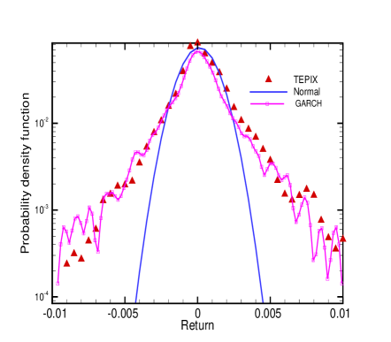
Figure 1: Comparison of the empirical probability distribution of TEPIX returns with the fitted normal distribution and GARCH(1,1) model.

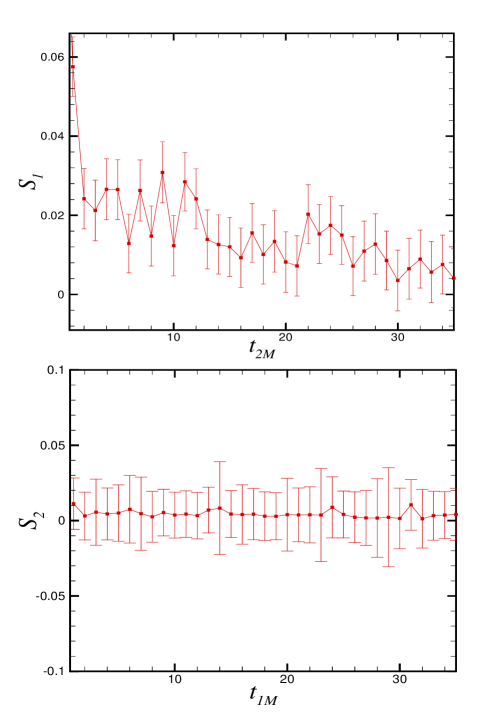
Figure 2: The $S$ values of daily prices of Brent Oil along with their statistical errors for return (upper graph) and volatilities (lower graph) in period 20 October 1985 to 24 September 2006.

Using this approach, we have considered some time series related to financial markets and commodities. We have calculated their Markov time scales for both returns and volatilities. Results are presented in Table 1. Taking into account results, indicates that Markov time scale of returns and volatilities for most of such data is equal 1. This implies that GARCH (1,1) model can be a well established model for financial modeling and descriptions. The calculated likelihood values for various GARCH ($q$,$p$) models support our approach. There is a good agreement between likelihood results and what Markov time scale approach suggests. Normally, the GARCH (1,1) model works better than other GARCH models and now it seems that the standard model has obtained another confirmation and could well capture the most important features of these kind of data in general. An interesting feature of our approach is that it works for both normal and fat-tail distributions. We have presented skewness, kurtosis and Hurst exponent values of selected time series in Table 1 to show statistical properties and fat-tailness of them jafari . They show different degrees of fat-tailness. Based on presented values in Table 1 the selected time series are far from normal distribution and have fat-tail distributions features and are very close to normal distributions. For normal distributions Hurst exponent is equal to 0.5 and greater exponents indicate fat-tailness. S&P500 and dow-jones indices together brent oil prices have lower degrees of fat-tailness compared to TEPIX and NZX. For a better comparison of the return distribution of TEPIX as an example of fat-tail distributions with a normal distribution and GARCH(1,1) model, the empirical PDF is presented in Fig.1 along with the fitted normal and GARCH(1,1) PDFs.

We have used above formalism for some daily time series such as $S\&P500$ (20 October 1982 to 24 November 2004), Dow-Jones( 4 January 1915 to 20 February 1990), New Zealand Exchange (NZX-7 January 1980 to 30 December 1999), Brent oil prices (4 January 1982 to 24 September 2006) and Tehran Price Index (TEPIX-20 May 1994 to 18 March 2004).

The value of $S$ in Eq. (3) has been calculated for two time series: returns and volatilities. In fig. 1 the results of $S$ values related to daily prices of Brent Oil along with their statistical errors for different time scales are shown. The interesting point is that our calculations show that Markov time scale for the daily return and volatility series in Brent oil prices is $q=1$ and $p=2$, respectively.

Table 1: The estimated values GARCH process parameters using Markov length scale approach

Time series	Skewness	Kurtosis	Hurst exponent	$q$	$p$
S$\&$P 500	1.93	45.10	0.44	1	1
Dow-Jones	-0.25	17.43	0.53	1	1
NZX	-1.43	27.29	0.61	1	1
TEPIX	0.72	18.50	0.74	1	1
Brent Oil	-1.25	34.99	0.51	2	1

In summary, we introduced a new criterion to find optimal $q$ and $p$ in GARCH family models. We have shown that a fundamental time scale in our approach is the Markov length, $t_{M}$, which is the minimum time interval over which the data can be considered as constituting a Markov process. This criterion support the success of standard GARCH (1,1) model to describe the majority of time series. In fact we suggest calculating Markov length for both return and volatility series to find proper parameters of GARCH models before proceeding to describe such processes and now we have a new method to select optimal $q$ and $p$ parameters in a GARCH ($q$, $p$) models.

IV acknowledgment

We would like to thank A. T. Rezakhani for his useful comments and discussions.

References

- (1) Engle R. F., (1982), Autoregressive conditional heteroskedasticity with estimates of the variance of U. K. in ation, Econometrica, 50, 987.
- (2) Bollerslev, T. (1986). Generalized autoregressive conditional heteroskedasticity. Journal of Econometrics 31, 307.
- (3) Bollerslev T, Engle R F and Nelson D B, ARCH models Handbook of Econometrics, vol 4, ed R F Engle and D M Mcfadden (1994).
- (4) Goodhart C. A. E. and Figliuoli L., (1991), Every minute counts in financial markets, Journal of International Money and Finance, 10, 23; Goodhart C. A. E., Hall S. G., Henry S. G. B., and Pesaran B., (1993), Journal of Applied Econometrics, 8, 113.
- (5) Goodhart C. A. E. and Hesse T., (1993), Central Bank Forex intervention assessed in continuous time, Journal of International Money and Finance, 12(4), 368.
- (6) Peiers B., (1994), A high-frequency study on the relationship between central bank intervention and price leadership in the foreign exchange market, unpublished manuscript, Department of Economics, Arizona State University.
- (7) Engle R. F., Ito T., and Lin W. L., (1990), Meteor showers or heat waves? Heteroskedastic intra-daily volatility in the foreign exchange market, Econometrica, 58, 525.
- (8) Baillie R. T. and Bollerslev T., (1990), Intra day and inter market volatility in foreign exchange rates, Review of Economic Studies, 58, 565.
- (9) Drost F. and Nijman T., (1993), Temporal aggregation of garch processes, Econometrica, 61, 909..
- (10) Andersen T. G. and Bollerslev T., (1994), Intraday seasonality and volatility persistence in foreign exhcnage and equity markets, Kellogg Graduate School of Management, Northwestern University, working paper 186, 1 30.
- (11) Bera A K and Higgins M L, ARCH models: properties, estimation and testing, J. Econ. Surv. 4 305 (1993).
- (12) Bollerslev, T. and Domowitz, I. (1993). Trading patterns and prices in the interbank foreign exchange market. Journal of Finance 48, 1421.
- (13) Pagan A.R. and Sabu H.,(1992), Consistency Tests for Hetroskedastic and Risk Models, Estudios Economics 7,30.
- (14) Solibakke P.B., Applied Financial Economics, Volume 11, Number 5,(2001), 539.
- (15) West K. D. and Cho D., (1994), The predictive ability of several models of exchange rate volatility, NBER technical working paper, 152, 1.
- (16) Friedrich R. and Peinke J., Phys. Rev. Lett. 78, 863 (1997); Friedrich R., et al., Phys. Lett. A 271, 217 (2000); Friedrich R., Peinke J., and Renner C., Phys. Rev. Lett. 84, 5224 (2000); Kriso S., et al., Phys. Lett. A 299, 287 (2002); Siegert S., Friedrich R. and Peinke J., Phys. Lett. A 243, 275 (1998); Jafari G. R., Fazeli S.M., Ghasemi F., Vaez Allaei S.M.,Reza Rahimi Tabar M., Irajizad A.,Kavei G., Phys. Rev. Lett. 91, 226101 (2003); Friedrich R., Zeller J., and Peinke J., Europhysics Letters 41, 153 (1998); Ghasemi F., Peinke J., Sahimi M. and Reza Rahimi Tabar M., Eur. Phys. J. B 47, 411 (2005).
- (17) Siefert M., Kittel A., Friedrich R. and Peinke J., Euro. Phys. Lett. 61, 466 (2003);
- (18) Bhattacharyya P. and Chakrabarti B. K. , Modelling Critical and Catastrophic Phenomena in Geoscience: A Statistical Physics Approach, (Springer, Berlin, 2006), p. 281;
- (19) Renner C, Peinke J, Friedrich R, Physica A 2001, 298, 211.
- (20) Risken H., The Fokker Planck Equation (Springer, Berlin, 1984)
- (21) Jafari G R, Movahed M S, Fazeli S M, Rahimi Tabar M Reza and Masoudi S F, J. Stat. Mech. (2006) P06008.