A Generalized Preferential Attachment Model
for Complex Systems

Abstract

Complex systems can be characterized by classes of equivalency of their elements defined according to system specific rules. We propose a generalized preferential attachment model to describe the class size distribution. The model postulates preferential growth of the existing classes and the steady influx of new classes. We investigate how the distribution depends on the initial conditions and changes from a pure exponential form for zero influx of new classes to a power law with an exponential cutoff form when the influx of new classes is substantial. We apply the model to study the growth dynamics of pharmaceutical industry.

working paper last revised:

Many diverse systems of physics, economics, and biology Barabasi ; Sergey ; City ; Zipf ; Satellite , share in their growth dynamics two basic similarities: (i) The system does not have a steady state and is growing. (ii) Basic units are born and they agglomerate to form classes. Classes grow in size preferentially depending on the existing size. In the context of economic systems, units are products, and the classes are firms. In social systems units are human beings, and the classes are cities. In biological systems units can be bacteria, and the classes are the bacterial colonies.

The probability distribution function $p(k)$ of the class size $k$ of the systems mentioned above share a universal behavior $p(k)\sim k^{-\tau}$ with $\tau\approx 2$ Barabasi ; City ; Zipf ; Kumar . Other possible values of $\tau$ are discussed and reported in Newman . Also, for most of the systems $p(k)$ has an exponential cutoff which is often assumed to be a finite size effect of the databases analyzed. Several models Sergey ; Champernowne ; Fedorowicz ; Gabaix ; Reed ; Simon explain $\tau\approx 2$ but none explains the exponential cutoff of $p(k)$. Moreover, these models describing $p(k)\sim k^{-\tau}$ are not suitable to describe simultaneously systems for which $p(k)\sim\exp(-\gamma k)$. Here we present a model with simple set of rules to describe $p(k)$ for the entire range of $k$, i.e., power law with an exponential cutoff. We show that the exponential cutoff of the power law is not due to finite size but an effect of the initial conditions from which the system starts to evolve. We also show that the functional form of $p(k)$ depends on the initial conditions of our model and changes from a pure exponential to a pure power law (with $\tau=2$) via a power law with an exponential cutoff. We justify our model by empirical analysis of a recently constructed pharmaceutical industry database (PHID) Pammolli ; Matia .

We now present a model, which has the following rules:

1. At time $t=0$ there exists $N$ classes, each with a single unit.

2. At each simulation step:

   • (a) With probability $b\ (0\leq b\leq 1)$ a class with a single unit is born.

   • (b) With probability $\lambda\ (0<\lambda\leq 1)$ a randomly selected class grows one unit in size. The selection of the class that grows is done with probability proportional to the number of units it already has [“preferential attachment”].

   • (c) With probability $\mu\ (0<\mu\leq 1,\mu<\lambda)$ a randomly selected class shrinks one unit in size. The selection of the class that shrinks is done with probability proportional to the number of units it already has [“preferential detachment”].

In the continuum limit the proposed growth mechanism gives rise to a master equation of $p(k,t_{i},t)$ which is the probability, for a class $i$ born at simulation step $t_{i}$, to have $k$ units at step $t$:.

$$\begin{split}&\frac{{\partial p(k,t_{i},t)}}{{\partial t}}=\lambda\frac{{(k-1)}}{{g(t)}}p(k-1,t_{i},t)\\ &+\mu\frac{{(k+1)}}{{g(t)}}p(k+1,t_{i},t)-(\lambda+\mu)\frac{k}{{g(t)}}p(k,t_{i},t)\end{split}$$ (1)

where $g(t)\equiv N+(\lambda-\mu+b)t$ is the total number of units at simulation step $t$ and $p(1,t_{i},t_{i})=1$. Equation (1) is the generalization of the master equation of birth and death processes Reed . The analytical solution of Eq. (1) is given by

$$p(k,t)=\frac{N}{{N+bt}}p(k,0,t),{\kern 10.0pt}+\frac{{b}}{{N+bt}}\int_{0}^{t}{dt_{i}{\kern 1.0pt}}p(k,t_{i},t)$$ (2)

where the functional form of $p(k,t_{i},t)$ is given in eqref . The lengthy derivation of the full solution of eq. 1 which is a power law(the second term of eq. 2) with an exponential cutoff (the first term of eq. 2) will be presented elsewhere, here we present simulation results.

First we discuss two limiting solutions of Eq. (1).

• Case i : No new classes are born ($b=0$). The growth of the system is solely due to the preferential attachment of new units to the pre-existing $N$ classes. In this case (Fig 1a) Reed

  $$p(k)\sim e^{-\frac{kN}{t(\lambda-\mu)}}.$$ (3)

  This limiting case can be considered as one of the initial condition of the model where birth or death of classes are not allowed. We observe that this initial condition results in a pure exponential distribution of the number of units inside classes.

• Case ii : At $t=0$, $N=0$, and new classes are born with probability $b\neq 0$. In this case, for large times $p(k)$ is a pure power law

  $$p(k)\sim k^{-\tau},\quad\tau=2.$$ (4)

  This limiting case can be considered as another different initial condition of the model where birth or death of classes are allowed starting from $N=0$ classes. We observe that this initial condition results in a pure power law distribution of the number of units inside classes.

  This case is identical to the Simon model Simon and can be understood by the following arguments. From case (i) we know that when the number of classes remains constant, $p(k)$ decays exponentially with $k$. The power law of case (ii) is the effect of superposition of many exponentials with different decay constants, each resulting from classes born at different times (Fig 1a).

We next present a mean field interpretation of the result $\tau\approx 2$. At any moment $t_{0}$ the number of units in the already-existing classes is $g(t_{0})$. Suppose a new class consisting of one unit is created at time $t_{0}$. According to rules 2b, 2c, the growth rate is proportional to $1/g(t_{0})$. Neglecting the effect of the influx of new classes on $g(t_{0})$, the average size $k$ of this class born at $t_{0}$ is proportional to $1/g(t_{0})$. So the classes which were born at times $t>t_{0}$ remain smaller than the classes born earlier. If we sort the classes according to their size, the rank $R(k)$ of a class is proportional to the time of its creation $R(k)\propto t_{0}$. Thus $k\sim 1/g(t_{0})\sim 1/t_{0}\sim 1/R(t_{0})$ and we arrive to the standard formulation of the Zipf’s law Zipf according to which the size of a class $k$ is inversely proportional to its rank. If we take into account the decrease of the growth rate with the influx of new classes, one can show after some algebra $k\sim R^{-(\lambda-\mu)/(\lambda-\mu+b)}$, which includes $k\sim R^{-1}$ as a limiting case for $b\rightarrow 0$. Since $R(k)$ is the number of classes whose size is larger than $k$, we can write in the continuum limit $R(k)\sim\int_{k}^{\infty}p(k)dk$ and hence $p(k)\sim k^{-2-b/(\lambda-\mu)}$.

The full solution of Eq. (1), a power law with an exponential cutoff, can be interpreted using the following arguments. We start with $N$ classes which are colored red, and let the newly born classes be colored blue. Due to the preferential attachment rule, the red classes remain on average larger than the blue classes. Thus for large $k$, $p(k)$ is governed by the exponential distribution of the red classes (Case i) while for small $k$, $p(k)$ is governed by the power law distribution of the blue classes (Case ii) (Fig. 1b).

Now we apply this model to describe the statistical properties of growth dynamics of business firms in pharmaceutical industry. PHID records quarterly sales figures of 48 819 pharmaceutical products commercialized in the European Union and North America from September 1991 to June 2001. The products in PHID can be classified in five different hierarchal levels A, B, C, D, and E (Fig. 2) note1 . Each level has a different number of classes, and different initial conditions (Table 1).

We observe that there are positive correlations between the number of units (products) appearing or disappearing per year and the number of units in the classes at a particular hierarchal level (Table 2). This empirical observation supports preferential birth or death mechanism (rules 2b, 2c) used in our model.

For levels A and B where the number of classes did not change we obtain an exponential distribution (Figs. 3a, 3b) as predicted by limiting Case i of the model. For levels C and D a weak departure from the exponential functional form [Figs. 3c, 3d] is due to the slight growth in the number of classes.

The full solution predicted by our model, i.e., the initial power law followed by the exponential decay of $p(k)$ is observed empirically for level E (Fig. 4). For level E we observe a power law with $\tau=1.97$ for $k<200$, and an exponential cutoff for $k>200$. From the discussion above with red and blue classes we may infer that the exponential part of $p(k)$ arises from pre-existing firms, while the power law part of $p(k)$ represents the young firms that enter the market. We conclude by noting that our model is in agreement with empirical observation where we observe $p(k)$ to be pure exponential or a power law with an exponential cutoff. Our analysis also sheds light on the emergence of the exponent $\tau\approx 2$ observed in certain biological, social and economic systems.

Level	A	B	C	D	E
total number of	13	84	259	432	3913
classes in each levels
number of classes	0	0	8	20	458
born in each level
number of classes	0	0	0	0	252
died in each level

Table 1: Two different initial conditions for classes in PHID levels: (i) For levels A and B we have no birth or death of classes. System grows with the birth or death of units to pre-existing $N$ classes (13 for level A and 84 for level B). (ii) For levels C and D system grows not only with the birth or death of classes but also with birth and death of units inside classes.

Level	A	B	C	D	E
correlation between number	0.93	0.87	0.84	0.82	0.70
of units born and existing
number of units in classes
correlation between number	0.88	0.86	0.80	0.78	0.75
of units died and existing
number of units in classes

Table 2: Correlation of birth and death of units with existing number of units in classes for each level in PHID. This observed correlation justifies the preferential birth or death of units which is rule 2 b and 2 c of our model.

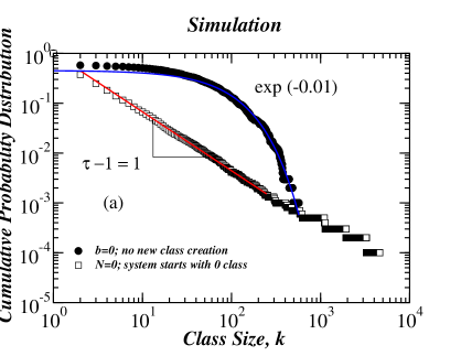
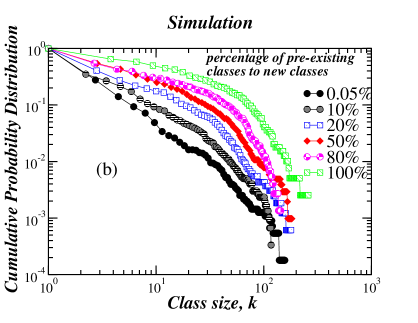
Figure 1: Simulation results of the model. (a) Symbols are data points from simulation, solid lines are regression fits. We observe for $b=0$ (i.e. no class creation ) cumulative probability distribution is a pure exponential while for $N=0$ (i.e. we start with zero initial class ) a pure power law $k^{-(\tau-1)}$ with exponent $\tau=2$. (b) We observe that as we change the ratio of number of pre-existing classes to the new born classes $p(k,t)$ changes from a pure power law to a pure exponential.

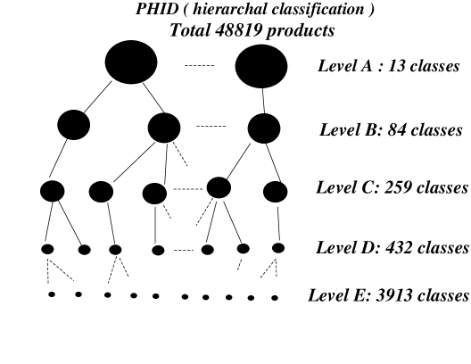
Figure 2: In the pharmaceutical industry, products can be classified according to five levels. When a particular product arrives in the market, it is labeled under any one of the 13 classes of the level A, 84 classes of level B, and so on. Since the 19th century, the number of classes of level A or B has remained constant even though the number of products within each class had a dramatic growth. Over the period of our empirical analysis the number of classes in levels C and D increased by 3% and 5% respectively. Products can also be grouped into firms which markets them (classification level E). In the figure we give the number of classes in each level in 1991.

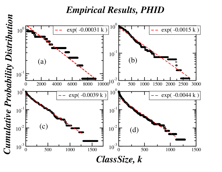
Figure 3: Figures (a)$\sim$(d) corresponds to levels (A)$\sim$(D) respectively. Products in the pharmaceutical industry are classified into levels A, B, C and D. Levels A and B have fixed numbers of classes, the number of classes in levels C and D increases by 3% and 5% respectively over the period of our analysis. For instance, for level A (fig. 3 a) which contains only 13 classes, the distribution is estimated from 13 random interger numbers which corresponds to classifying 48,819 products in 13 classes. Symbols represent data points in each level (a)$\sim$(d) while solid lines are predictions of the model. Cumulative probability distributions for all levels are pure exponentials as predicted by the model.

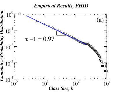
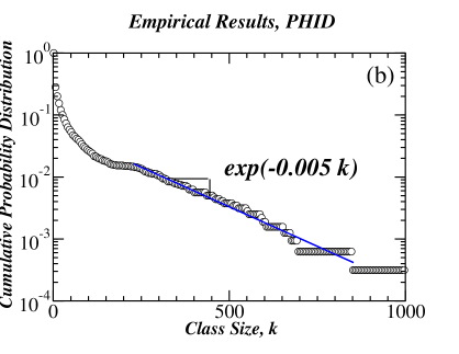
Figure 4: Empirical results from PHID level E. The classes analyzed here are the firms. Circles are data points, solid lines are regression fits. (a) Log-log plot of cumulative probability distribution of the class sizes show a power law decay $k^{-(\tau-1)}$ with $\tau\approx 2$ for $k<200$. (b) Log-linear plot of cumulative probability distribution show the exponential decay for $k>200$.

References

- (1) H. Jeong, B. Tomber, R. Albert, Z. N. Oltvai, and A. L. Barabási, Nature 407, 651 (2000).
- (2) S. V. Buldyrev, N. V. Dokholyan, S. Erramilli, M. Hong, and J. Y. Kim et al., Physica A 330, 653 (2003).
- (3) M. Batty and P. Longley, Fractal Cities (Academic Press, San Diego, 1994).
- (4) G. Zipf, Human behavior and the principle of last effort (Addison-Wesley, Cambridge, 1949).
- (5) H. A. Makse, J. S. Andrade, M. Batty, S. Havlin, and H. E. Stanley, Phys. Rev. E 58, 7054 (1998).
- (6) R. Kumar, P. Raghavan, S. Rajagopalan, and A. Tomkins, Comput. Netw. 31, 1481 (1999).
- (7) M. E. J. Newman, preprint condmat/0412004.
- (8) , and
- (9) D. Champernowne, Economic Journal 63, 318 (1953).
- (10) J. Fedorowicz, Journal of American Society of Information Science 33, 223 (1982).
- (11) X. Gabaix (1999), Quarterly Journal of Economics 114, 739 (1999).
- (12) W. J. Reed and B. D. Hughes, Phys. Rev. E 66, 067103 (2002).
- (13) Y. Ijiri and H. A. Simon, Skew distributions and the sizes of business firms (North-Holland Pub. Co., Netherlands, 1977).
- (14) G. De Fabritiis, F. Pammolli, M. Riccaboni, Physica A 324, 38 (2003).
- (15) K. Matia, D. Fu, S. V. Buldyrev, F .Pammolli, M. Riccaboni and H. E. Stanley EPL 67 498 (2004).
- (16) The different levels A, B, C, D of PHID are the four different anatomical therapeutic chemical (ATC) levels. Classes in ATC 1 are organs of the body, classes in ATC 2 are therapeutic preparations, classes in ATC 3 and 4 are the chemicals and compounds respectively used in preparing the products. For level E the classes are the firms like Merck, Glaxo etc.