Statistical Properties of Business Firms Structure and Growth

Abstract

We analyze a database comprising quarterly sales of 55624 pharmaceutical products commercialized by 3939 pharmaceutical firms in the period 1992–2001. We study the probability density function (PDF) of growth in firms and product sales and find that the width of the PDF of growth decays with the sales as a power law with exponent $\beta=0.20\pm 0.01$. We also find that the average sales of products scales with the firm sales as a power law with exponent $\alpha=0.57\pm 0.02$. And that the average number products of a firm scales with the firm sales as a power law with exponent $\gamma=0.42\pm 0.02$. We compare these findings with the predictions of models proposed till date on growth of business firms.

In economics there are unsolved problems that involve interactions among a large number of subunits [1, 2, 3]. One of these problems is the structure of a business firm and its growth [2, 4]. As in many physical models, decomposition of a firm into its constituent parts is an appropriate starting place for constructing a model. Indeed, the total sales of a firm is comprised of a large number of product sales. Previously accurate data on the “microscopic” product sales have been unavailable, and hence it has been impossible to test the predictions of various models. Here we analyze a new database, the Pharmaceutical Industry Database (PHID) which records quarterly sales figures of 55624 pharmaceutical products commercialized by 3939 firms in the European Union and North America from September 1991 to June 2001. We shall see that these data support the predictions of a simple model, and at the same time the data do not support the microscopic assumptions of that model. In this sense, the model has the same status as many statistical physics models, in that the predictions can be in accord with data even though the details of microscopic interactions are not. The assumptions of this simple model given in Ref [5] are as follows: (i) Firms tends to organize itself into multiple divisions once they attain a particular size. (ii) The minimum size of firms in a particular economy comes from a broad distribution. (iii) Growth rates of divisions are independent of each other and there is no temporal correlation in their growth. With these assumptions the model builds a diversified multi-divisional structure. Starting from a single product evolving to a multi-product firm, this model reproduces a number of empirical observations and make some predictions which we discuss in detail below along with results and predictions of other models which attempt to address the problem of business firm growth.

Consider a firm $i$ of sales $S_{i}$ with $N_{i}$ products whose sales are $\xi_{i,j}$ where $j=1,2,...,N_{i}$. Thus the firm size in terms of the sales of its products is given as $S_{i}=\sum_{j=1}^{j=N_{i}}\xi_{i,j}$. The growth rate is

$$g_{i}(t)\equiv\log\left(\frac{S_{i}(t+\Delta t)}{S_{i}(t)}\right)=\log S_{i}(t+\Delta t)-\log S_{i}(t),$$ (1)

where $S_{i}(t)$ and $S_{i}(t+\Delta t)$ are the sales, in units of $10^{3}$ British Pounds, of firm $i$ being considered in the year $t$ and $t+\Delta t$, respectively. Pharmaceutical data has seasonal effect, and hence the analysis of quarterly data will have effects due to seasonality. To remove any seasonality, that might be present, we analyze the annual data instead of the quarterly data.

Recent studies have demonstrated power-law scaling in economic systems [6]. In particular the standard deviation $\sigma$ of the growth rates of diverse systems including firm sales  [6] or gross domestic product (GDP) of countries [7] scales as a power-law of $S$.

The models of Refs [1, 5, 8, 2, 3] all predicts that standard deviation of growth rates amongst all firms with the same sales scales as a power law $\sigma(g|S)\sim S^{-\beta}$. Further, model of Refs [5] predicts that probability density function PDF $p(g|S)$, of growth rates for a size of firm $S$ scales as a function of $S$ as :

$$p(g|S)\sim\frac{1}{S^{-\beta}}~{}~{}f_{0}\left(\frac{g}{S^{-\beta}}\right)\,\,$$ (2)

where $f_{0}$ is a symmetric function of a specific “tent-shaped” form resulting from a convolution a log normal distributions and a Gaussian distribution, with parameters dependent on the parameters of the model. Figure 1a plots the scaling of the standard deviation $\sigma(g|S)$. We observe $\sigma(g|S)\sim S^{-\beta}$ with $\beta=0.19\pm 0.01$. Figure 1b plots the scaled PDF as given by eq. 2 for three sales groups; small ($S<10^{2}$), medium ($10^{2}<S<10^{4}$) and large ($10^{4}<S$). The figure also plots $f_{0}$ as predicted by refs [5].

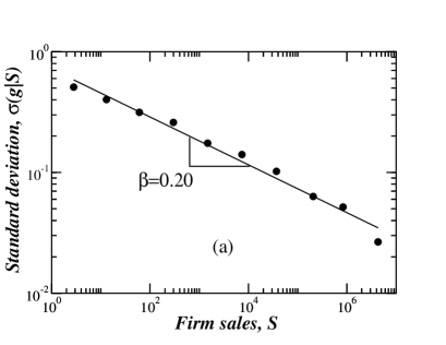
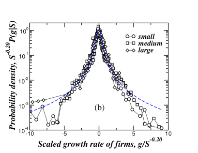
Figure 1: (a) Firms are divided into 10 groups according to firm sale $S$. We find the standard deviation $\sigma(g|S)$ of the growth rates scales as a power law, $\sigma(g|S)\sim S^{-\beta}$ with $\beta=0.20\pm 0.01$. Symbols are data points and solid line is a regression fit. (b) PDF of the growth rates for small [$S<10^{2}$], medium [$10^{2}<S<10^{4}$], and large [$10^{4}<S$] values of S is scaled by their standard deviation. Note the collapse of the histograms of the three groups which confirms the scaling exponent $\beta$. The dashed line is $f_{0}$ as predicted by the model approximating the results of ref  [5] given by $f_{0}(x)\approx a_{0}\exp\{(-a_{1}~{}(1+0.75~{}\ln(1+a_{2}~{}x^{2})]\}[1+0.75~{}\ln(1+a_{2}~{}x^{2})]^{1/2}$ where $a_{0},~{}a_{1}$,and $a_{2}$ are parameters of the model.

The model of Ref [5] further predicts that the PDF of the product size $\xi$ for a fixed firm size $S$, $\rho_{1}(\xi|S)$ should scale as

$$\rho_{1}(\xi|S)\sim\frac{1}{S^{\alpha}}~{}~{}f_{1}\left(\frac{\xi}{S^{\alpha}}\right)\,.$$ (3)

where again $f_{1}$ depends on the parameters of the model. According to the model discussed in Refs [5, 8] $f_{1}$ is a log-normal PDF. We then evaluate the average product size $E(\xi|S)$ in a firm of size $S$, defined as $E(\xi|S)=\int d\xi\rho_{1}(\xi|S)\xi\sim S^{\alpha}$. Figure 2b plots $E(\xi|S)$, we observe $E(\xi|S)\sim S^{\alpha}$ with $\alpha=0.57\pm 0.02$. Figure 2b plots the scaled PDF as given by eq. 3 for three sales groups; small ($S<10^{2}$), medium ($10^{2}<S<10^{4}$) and large ($10^{4}<S$). We observe that for each of the groups the PDF $\rho_{1}(\xi|S)$ is consistent with a log-normal distribution by noting in a log-log plot the PDF $\rho_{1}(\xi|S)$ is parabolic which is tested by performing a regression fit.

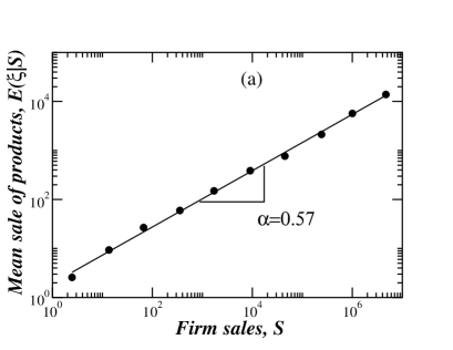
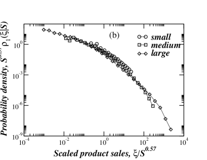
Figure 2: (a) Mean, $E(\xi|S)$ of the product sale conditioned for a firm of sale $S$. We observe that the mean scales as $E(\xi|S)\sim S^{\alpha}$ with $\alpha=0.57\pm 0.02$. Symbols are data points and solid line is a regression fit. (b) PDF of the product sales for small [$S<10^{2}$], medium [$10^{2}<S<10^{4}$], and large [$10^{4}<S$] values of S scaled by $S^{0.57}$. Note the collapse of the PDF’s of the three groups which confirms the scaling exponent $\alpha$.

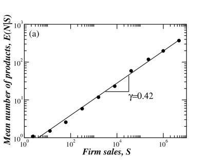
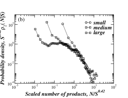
Figure 3: (a) Mean, $E(N|S)$ of the number of products $N$ for a firm of sale $S$. Symbols are data points and solid line is a regression fit. We observe that the mean scales as $E(N|S)\sim S^{\gamma}$ with $\gamma=0.42\pm 0.01$.(b) PDF of the number of product for small [$S<10^{2}$], medium [$10^{2}<S<10^{4}$], and large [$10^{4}<S$] values of S scaled by $S^{0.42}$. Note the partial collapse of the PDF’s for of the three groups which confirms the scaling exponent $\gamma$. For small values of $N$, which also corresponds to small values of $S$, the statistics become poor. This statistical errors gets even more amplified when we divide small values of $N$ by $S^{0.42}$. Thus we observe poor quality of data collapse for $N/S^{0.42}<1$. The data collapse is better for $N/S^{0.42}>1$ where we have good statistics.

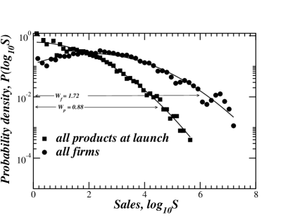
Figure 4: PDF of products sales (diamond) firm sales (circles) between 1990-2001. The variance of the PDF’s of products sales at launch and firm sales are estimated to be $W_{p}=0.88$ and $W_{f}=1.72$ respectively. This gives $W_{f}-W_{p}=0.84$ and $\beta=0.24$ [cf. eq. 7] which is approximately what is observed empirically as predicted by [5].

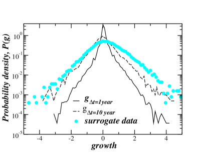
Figure 5: Probability density function (PDF), $P(g_{\Delta t})$ of products for ${\Delta t}=1$ year (solid line) and ${\Delta t}=10$ years (dashed line). Circles represent the of surrogate data [9]. In absence of correlation we expect the data for $\Delta t=10$ to coincide with the PDF of the surrogate points.

According to Ref [5], the PDF $\rho_{2}(N|S)$ of number of products $N$ in a firm of size $S$ should obey the scaling relation:

$$\rho_{2}(N|S)\sim\frac{1}{S^{\gamma}}~{}~{}f_{2}\left(\frac{N}{S^{\gamma}}\right)\,.$$ (4)

where the function $f_{2}$ is log-normal and depends of the parameters of the model. We evaluate the average number of products $E(N|S)$ for a firm of size $S$. Using eq. 4 we note that $E(N|S)=\int dN\rho_{1}(N|S)N\sim S^{\gamma}$. Figure 3a plots the expectation $E(N|S)$ and we observe that $E(N|S)\sim S^{\gamma}$ with $\gamma=0.42\pm 0.01$. Figure 3b plots the scaled PDF $\rho_{2}(N|S)$ as given by eq. 4 for three groups; small ($S<10^{2}$), medium ($10^{2}<S<10^{4}$) and large ($10^{4}<S$) .

According to [5] the relations between the scaling exponents $\alpha~{}\beta$, and $~{}\gamma$ are given by

$$\gamma = 1-\alpha,$$ (5)

$$\beta = \frac{1-\alpha}{2}$$ (6)

which we find to be approximately valid for the PHID database.

According to the model discussed in refs [5], the distribution of product sizes in each firm scales with the product size at launch $S_{\mathrm{at~{}launch}}$, according to, $\rho_{0}(\xi/S_{\mathrm{at~{}launch}})$ which is approximately log-normal. Model [5] postulates that the PDF of $S_{\mathrm{atlaunch}}$ is log normal, i.e., $P(\log S_{\mathrm{at~{}launch}})$ is Gaussian with variance $W_{p}$ and each firm is characterized by a fixed value of $S_{\mathrm{at~{}launch}}$. Furthermore, ref. [5] predicts that the distribution of firm sales is close to log normal i.e., the PDF $P(\log S)$ is Gaussian with variance $W_{f}$. With these hypothesis ref. [5] derives that,

$$\beta=\frac{W_{f}-W_{p}}{2~{}W_{f}}.$$ (7)

Figure 4 plots PDF of annual products sales, products sales at launch $P(\log S_{\mathrm{at~{}launch}})$, and firm sales $P(\log S)$ between 1990-2001. The variance of the PDF’s of products sales at launch and firm sales are estimated to be $W_{p}=0.88$, $W_{f}=1.72$ respectively. This gives $\beta=(W_{f}-W_{p})/2~{}W_{f}=0.24$ which is approximately what is observed empirically. We employ two methods to estimate $W$ (the standard deviation) : (i) Estimate $W$ from the definition, i.e. $W^{2}=(1/(N-1))\sum_{i=1}^{i=N}(x_{i}-<x>)^{2}$ where $\{x_{1},x_{2},...x_{N}\}$ is a set of data and $<x>$ is the mean of the set $\{x_{i}\}$. (ii) First estimate the PDF from the set $\{x_{i}\}$, then perform a regression fit with a log-normal function to the PDF. The standard deviation $W$ will be one of the fitting parameter. Hence estimate $W$ from the estimated parameter value from the least square log-normal fit to the PDF. We observe both this method gives similar values of $W$ and the ratio $\beta$ (cf. eq.7 ) remains unchanged as long as we consistently use one of the 2 methods described above. Our estimate of $W$ presented here is using the former method.

Ref. [5] postulates products growth rate to be Gaussian and temporally uncorrelated. To test this postulate figure 5 plots the PDF $P(g)$ of the growth $g$ of the products $\Delta t=1$ and $\Delta t=10$ year [9]. We see that the empirical distribution is not growing via random multiplicative process as ref. [5] postulates but has the same tent shape distribution as the distribution of firm sales growth rate, suggesting that the products themselves may not be elementary units but maybe comprised of smaller interacting subunits. Figure 5 also plots PDF $P(g^{\prime})$ surrogate data obtained by summation of the 10 annual growth rates from the empirical distribution. We observe that the $P(g_{\Delta t=10})$ for products differs from the surrogate data implying there are significant anti-correlation in the growth dynamics between successive years.

In summary we study the statistical properties of the internal structure of a firm and its growth. We identify three scaling exponents relating the (i) sales of the products, $\xi$ (ii) the number of products, $N$ and (iii) the standard deviation of the growth rates, $\sigma$, of a firm with its sales $S$. Our analysis confirms the features predicted in ref [5]. However we find that the postulate of the model namely: the growth rate of the products is uncorrelated and Gaussian is not accurate. Thus the model of ref. [5] can be regarded as a first step towards the explanation of the dynamics of the firm growth.

We thank L. A. N. Amaral, S. Havlin for helpful discussions and suggestions and NSF and Merck Foundation (EPRIS Program) for financial support.

References

- [1] Y. Ijiri and H.A. Simon, Skew Distributions and the Sizes of Business Firms (North-Holland, Amsterdam, 1997).
- [2] J. Sutton, PHYSICA A, 312, 577 (2002).
- [3] M. Wyart and J.P. Bouchaud, cond-math/0210479v2 (19 Nov 2002).
- [4] R. H. Coase, Economica 4, 386 (1937); R. H. Coase The Nature of Firm: Origins, Evolution and Development. (Oxford University Press, New York, 1993), 34-74; E. Mansfield, Research Policy 20, 1 (1991); A. Pakes and K. L. Sokoloff, Proc. Nat. Ac. Sci. USA 93, 12655 (1996); R. Erikson, A. Pakes, Rev. of Eco. Studies 62, 53 (1995).
- [5] L. A. N. Amaral, S. V. Buldyrev, S. Havlin, M. A. Salinger, and H. E. Stanley, Phys. Rev. Lett. 80, 1385 (1998).
- [6] M. H. R. Stanley, L. A. N. Amaral, S. V. Buldyrev, S. Havlin, H. Leschhorn, P. Maass, M. A. Salinger, and H. E. Stanley, Nature (London) 379, 804 (1996); L. A. N. Amaral, S. V. Buldyrev, S. Havlin, H. Leschhorn, P. Maass, M. A. Salinger, H. E. Stanley, and M. H. R. Stanley , J. Phys. I (France) 7, 621 (1997); S. V. Buldyrev, L. A. N. Amaral, S. Havlin, H. Leschhorn, P. Maass, M. A. Salinger, H. E. Stanley, and M. H. R. Stanley, J. Phys. I (France) 7, 635 (1997); Y Lee, L. A. N. Amaral, D. Canning, M. Meyer, and H. E. Stanley. Phy. Rev. Lett. 81, 3275 (1998); D. Canning, L. A. N. Amaral, Y. Lee, M. Meyer, and H. E. Stanley, Economics Letters 60, 335 (1998); T. Keitt and H. E. Stanley, Nature (London) 393, 257 (1998).
- [7] V. Plerou, L. A. N. Amaral, P. Gopikrishnan, M. Meyer, and H. E. Stanley, Nature (London) 400, 433 (1999).
- [8] G. De Fabritiis, G. Pammolli, M. Riccaboni, PHYSICA A 324, 38 (2003).
- [9] . And .
- [10] H. E. Stanley, Reviews of Modern Physics 71, S358 (1999).