Time and Frequency description of Optical Pulses

Abstract

The connection between the time-dependent physical spectrum of light and the phase space overlap of Wigner functions is investigated for optical pulses. Time and frequency properties of optical pulses with chirp are analyzed using the phase space Wigner and Ambiguity distribution functions. It is shown that optical pulses can exhibit interesting phenomena, very much reminiscent of quantum mechanical interference, quantum entanglement of wave packets, and quantum sub-Planck structures of the time and frequency phase space.

I Introduction

In a paper published in 1977, Professor Eberly and one of the present authors (KW), have introduced the time-dependent physical spectrum of light described by non-stationary random electric fields jhekw1977 . The definition of such an operational spectrum required, as an essential step, a frequency tunable filter, that allows the resolution of the frequency components. If one restricts the result of jhekw1977 to deterministic fields only, the time-dependent physical spectrum takes the following form

$$G(t,\omega)=\biggl{|}\int ds\,{\mathcal{J}(t-s;\Gamma)E(s)e^{i\omega s}}\biggl{|}^{2}\,,$$ (1)

where $E(t)$ is the positive frequency part of the detected electric field, and the spectral properties of the filter are represented by the response function $\mathcal{J}(t;\Gamma)e^{i\omega t}$. This function depends on the setting frequency $\omega$, and the response amplitude is characterized by a bandwidth $\Gamma$ of the filter. If one rewrites the time-dependent spectrum formula (1) in the following form

$$G(t,\Gamma)=\biggl{|}\int ds\,{\mathcal{J}\bigl{(}\frac{t-s}{\Gamma}\bigr{)}E(s)e^{i\omega s}}\biggl{|}^{2}\,,$$ (2)

and look at (1) as a function of time and bandwidth only, we recognize in this expression the modulus square of the wavelet transformation of the signal field, where $t$ is the time shift and $\Gamma$ is the scale mallat1999 .

Several years after the introduction of the time-dependent spectrum, similar expressions to (1) have been derived and applied to the reconstruction of the amplitude and phase of optical pulses. If one selects $\mathcal{J}(t)=|E(t)|^{2}$ or $\mathcal{J}(t)=E(t)$, the recorded time-dependent spectrum corresponds to the frequency resolved optical gating (FROG) frog1993 , or to the second harmonic frequency resolved optical gating (SHG FROG) frog1994 . Methods based on FROG have become powerful tools in the investigations of femtosecond pulses.

The remarkably simple expression (1), hides a very interesting phase space structure of the operational spectrum in terms of a time and frequency distribution overlap. It has been shown kbkw1982 , that the time-dependent spectrum can be visualized as a time and frequency convolution of two Wigner distribution functions

$$G(t,\omega)=2\pi\int dt^{\prime}\int d\omega^{\prime}\,W_{J}(t^{\prime},\omega^{\prime})W_{E}(t^{\prime}+t,\omega^{\prime}+\omega)\,.$$ (3)

In this expression the first Wigner function corresponds to the time and frequency distribution of the filter, while the second Wigner function describes the phase space properties of the measured electric field. It is perhaps worth mentioning, that a quantum version of the expression (3), can be applied in quantum mechanics, to describe joint operational measurements of position and momentum kw1984a .

In order to honor Professor Eberly’s contributions to the development of the time-dependent spectrum and Quantum Optics, this paper will investigate time and frequency properties of optical pulses using the concept of the phase space Wigner distribution. We will show that optical pulses can exhibit interesting phase space structures very much reminiscent of quantum mechanical interference cgplk2005 , quantum entanglement of wave packets laweberly2004 , and quantum sub-Planck structures zurek2001 .

This paper is organized in the following way. Section II is devoted to the definition and elementary properties of the time and frequency Wigner and Ambiguity distribution functions. Section III contains a detailed description of chirped pulses using a time and frequency phase space. We show that time and frequency correlations of chirped pulses have a formal analogy to entanglement of wave packets. The strength of these correlations is investigated using the Schmidt decomposition. In Section IV we analyze the phase space properties of a linear superposition of two chirped pulses. In Section V we discuss the connection of sub-Fourier phase space structures with pulse overlaps. Finally some concluding results are presented.

II Time and Frequency Phase Space

II.1 The Wigner Function

We shall investigate time and frequency properties of optical pulses using a phase space distribution function. Such a function has been originally introduced by Wigner in 1932 and applied to quantum mechanics wigner1932 . In the area of signal processing the same distribution function has been used by Ville in 1948 ville1948 . The time and frequency Wigner distribution function corresponding to the field envelop $E(t)$ is defined as

$$W_{E}(t,\omega)=\int\frac{ds}{2\pi}\;E^{\ast}\left(t+\frac{s}{2}\right)\;e^{i\omega s}\;E\left(t-\frac{s}{2}\right)\,.$$ (4)

It is well known that the Wigner function can be used as a time and frequency distribution of the pulse, but cannot be guaranteed to be positive for all fields. There is an extensive literature devoted to the properties and applications of the Wigner function in quantum mechanics schleich2001 and classical optics cohen1995 . Below we present only the most relevant properties of the Wigner distribution needed for the purpose of this paper.

The frequency integration of the Wigner function yields the temporal instantaneous intensity

$$\int d\omega\,W_{E}(t,\omega)=I(t)=E^{\ast}(t)E(t)\,.$$ (5)

The corresponding time integration of this distribution leads to the power spectrum of the optical pulse

$$\int dt\,W_{E}(t,\omega)=P(\omega)=\frac{1}{2\pi}\tilde{E}^{\ast}(\omega)\tilde{E}(\omega)\,.$$ (6)

In this formula the expression $\tilde{E}(\omega)=\int dte^{-i\omega t}E(t)$ is the Fourier transform of the pulse. From these definitions we see that that the Wigner function is normalized to the total power/energy of the pulse

$$\int dt\int d\omega\,W_{E}(t,\omega)=\int dt\,I(t)=\int d\omega\,P(\omega)\,,$$ (7)

where the last equality follows from the Parseval theorem for the Fourier transforms. An important result that we shall use in the following sections is the overlap relation for two Wigner functions

$$|\langle E_{1}|E_{2}\rangle|^{2}=\left|\int dtE^{\ast}_{1}(t)E_{2}(t)\right|^{2}=2\pi\int dt\int d\omega\,W_{E_{1}}(t,\omega)W_{E_{2}}{(}t,\omega)\,.$$ (8)

This formula indicates that the case a zero overlap of two pulses is impossible to achieve with positive Wigner functions.

Using the Wigner function as a weighting distribution one can characterize the properties of the optical pulse in the form of the following statistical moments of time and frequency

$$\langle t^{n}\omega^{m}\rangle=\frac{\int dt\int d\omega\,t^{n}\omega^{m}\,W_{E}(t,\omega)}{\int dt\int d\omega\,W_{E}(t,\omega)}\,.$$ (9)

II.2 The Ambiguity function

A different way of looking at the time-frequency correlations (9) is to use the Ambiguity function, which is a two-dimensional Fourier transform of the Wigner function

$$A_{E}(T,\Omega) = \int dt\int d\omega\,e^{i\Omega t+i\omega T}W_{E}(t,\omega)$$ (10)

$$= \int dt\;E^{\ast}\left(t-\frac{T}{2}\right)\;e^{i\Omega t}\;E\left(t+\frac{T}{2}\right)\,.$$

From this definition it follows that the Ambiguity function can be written as

$$A_{E}(T,\Omega)=A_{E}(0,0)\langle e^{i\Omega t+i\omega T}\rangle\,,$$ (11)

where $A_{E}(0,0)=\int dt\int d\omega\,W(t,\omega)$ is a normalization constant. The formula (11) can be used as a moment generating function. The time and frequency statistical moments (9) can be calculated from the Ambiguity function using the formula

$$\langle t^{n}\omega^{m}\rangle=\frac{(-i)^{n+m}}{A_{E}(0,0)}\frac{d^{n}}{d\Omega^{n}}\frac{d^{m}}{dT^{m}}A_{E}(T,\Omega)\biggl{|}_{T=\Omega=0}\,.$$ (12)

II.3 ABCD optics of optical pulses

It is known from classical optics that for linear optical devices one can use the $ABCD$ transformation of geometrical ray displacement and slope pmjhe . We will use this approach to describe arbitrary linear transformations of time and frequency given by

$$\left(\begin{array}[]{c}t^{\prime}\\ \omega^{\prime}\\ \end{array}\right)=\left(\begin{array}[]{cc}A&B\\ C&D\\ \end{array}\right)\left(\begin{array}[]{c}t\\ \omega\\ \end{array}\right)\,.$$ (13)

This transformation is canonical if it preserves the normalization of the Wigner function

$$\int dt\int d\omega\,W(At+B\omega,Ct+D\omega)=\int dt\int d\omega\,W(t,\omega)\,.$$ (14)

This condition is satisfied if

$$\det\left(\begin{array}[]{cc}A&B\\ C&D\\ \end{array}\right)=1\,.$$ (15)

The $ABCD$ transformation of the Wigner function generates the following transformation of the Ambiguity function

$$W(At+B\omega,Ct+D\omega)\Rightarrow A_{E}(At-B\omega,D\omega-Ct)\,.$$ (16)

III Time and frequency description of chirped pulses

III.1 General properties of chirped pulses

Let us write the electric field in the form of a real envelop and phase:

$$E(t)=\mathcal{E}(t)e^{-i\varphi(t)}\,.$$ (17)

In order to calculating the Wigner function for such a pulse we use a linear approximation for the phase: $\varphi(t+s/2)-\varphi(t-s/2)\simeq\dot{\varphi}s$, and as a result we obtain

$$W_{E}(t,\omega)=W_{\mathcal{E}}(t,\omega+\dot{\varphi})\,,$$ (18)

where $W_{\mathcal{E}}(t,\omega)$ is the Wigner function of the real envelop $\mathcal{E}(t)$. The corresponding formula for the Ambiguity function is

$$A_{E}(t,\omega)=A_{\mathcal{E}}(t,\omega-\dot{\varphi})\,.$$ (19)

The instantaneous pulse frequency $\omega(t)$ of a chirped pulse $E(t)=\mathcal{E}(t)e^{i\omega(t)}$, can be defined as

$$\omega(t)=\frac{\int d\omega\,\omega\,W_{E}(t,\omega)}{\int d\omega\,W_{E}(t,\omega)}=\langle\omega\rangle_{\mathcal{E}}-\dot{\varphi}\,,$$ (20)

and the corresponding square of instantaneous pulse frequency is

$$\omega^{2}(t)=\frac{\int d\omega\,\omega^{2}\,W_{E}(t,\omega)}{\int d\omega\,W_{E}(t,\omega)}=\langle\omega^{2}\rangle_{\mathcal{E}}-2\dot{\varphi}\langle\omega\rangle_{\mathcal{E}}+\dot{\varphi}^{2}\,,$$ (21)

where $\langle\omega\rangle_{\mathcal{E}}$ and $\langle\omega^{2}\rangle_{\mathcal{E}}$ are the frequency two moments, calculated with respect to the unchirped amplitude $\mathcal{E}$. From these relations we conclude that the dispersion of the instantaneous pulse frequency is

$$(\Delta\omega(t))^{2}=(\Delta\omega)_{\mathcal{E}}^{2}+(\Delta\dot{\varphi}(t))^{2}\,.$$ (22)

III.2 Gaussian optical pulses with linear chirp

As an example of the general envelop (17), we will consider a single pulse with a linear chirp and Gaussian envelop function of the form

$$E(t)=\exp\left(-i\omega_{l}t-\frac{t^{2}}{4\sigma^{2}}(1+ia)\right)\,.$$ (23)

We have assumed that our pulse is long enough, so one can perform the standard decomposition of the electric field into the slow amplitude (17), and the harmonic carrier with frequency $\omega_{l}$. The intensity and the power spectrum of this pulse are

$$I(t)=\exp\left(-\frac{t^{2}}{2\sigma^{2}}\right),\quad P(\omega)=\frac{2\sigma^{2}}{\sqrt{1+a^{2}}}\exp\left(-\frac{2\omega^{2}\sigma^{2}}{1+a^{2}}\right)\,.$$ (24)

In these formulas the full duration of the pulse is defined as a full width at half maximum of the intensity (FWHM): $\tau_{p}=2\sqrt{2\ln 2}\,\sigma$, the linear chirp is characterized by a real parameter $a$, and the electric field amplitude has been conveniently selected to be one in arbitrary units. In all numerical applications in this paper, we select $\sigma^{2}=1/2$ leading to a pulse duration $2\sqrt{\ln 2}$. In order to keep our formulas simple we have shifted the frequency $\omega$ in such a way that it incorporates the constant carrier frequency.

The chirp on the pulse (23) corresponds to a linear chirp $\dot{\varphi}(t)=\frac{a}{2\sigma^{2}}t$, leading to the instantaneous pulse frequency $\omega(t)=-\frac{a}{2\sigma^{2}}t$. For the Gaussian pulse the formula (22) becomes

$$(\Delta\omega)^{2}=\frac{1}{4\sigma^{2}}+\frac{a^{2}}{4\sigma^{2}}\langle t^{2}\rangle\,.$$ (25)

We see that the linear chirp is equivalent to a transformation given by the following $ABCD$ matrix

$$\left(\begin{array}[]{cc}A&B\\ C&D\\ \end{array}\right)=\left(\begin{array}[]{cc}1&0\\ \frac{a}{2\sigma^{2}}&1\\ \end{array}\right)\,.$$ (26)

This matrix has the typical form for a ray transformation due to a thin lens pmjhe .

Let us investigate the time and frequency properties of the chirped pulse. Simple calculation shows that the Wigner function of this pulse is

$$W(t,\omega) = W_{0}\bigl{(}t,\omega+\frac{a}{2\sigma^{2}}t\bigr{)}$$ (27)

$$= \frac{2\sigma}{\sqrt{2\pi}}\exp\left(-\frac{t^{2}}{2\sigma^{2}}(1+a^{2})-2\omega^{2}\sigma^{2}-2a\omega t\right)\,,$$

where $W_{0}(t,w)=\frac{2\sigma}{\sqrt{2\pi}}\exp\left(-\frac{t^{2}}{2\sigma^{2}}-2\omega^{2}\sigma^{2}\right)$ is the Wigner function of a Gaussian pulse with no chirp. In Figures (1) and (2) we have depicted the Wigner function of a Gaussian pulse with no chirp and chirp $a=3$.

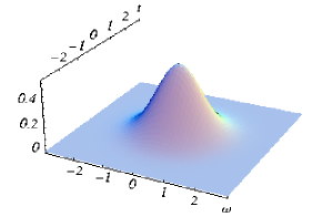
Figure 1: Plot of the Wigner function for a Gaussian pulse with pulse duration $\tau_{d}=2\sqrt{\ln 2}$ and no chirp ($a=0$).

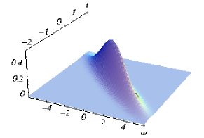
Figure 2: Plot of the Wigner function for a Gaussian pulse with pulse duration $\tau_{d}=2\sqrt{\ln 2}$ and chirp $a=3$.

For the Ambiguity function a simple calculation for the chirped pulse gives an expression similar to the formula (27)

$$A_{E}(T,\Omega) = A_{E}(0,0)A_{0}(T,\Omega-\frac{a}{2\sigma^{2}}T)$$ (28)

$$= A_{E}(0,0)\exp\left(-\frac{T^{2}}{8\sigma^{2}}(1+a^{2})-\frac{\Omega^{2}\sigma^{2}}{2}+\frac{a}{2}T\Omega\right)\,.$$

This function can be written as a general Gaussian function of two variables

$$A_{E}(T,\Omega)=A_{E}(0,0)\exp\left(-\frac{1}{2}\mathbf{v}\,\mathbf{C}\,\mathbf{v}^{T}\right)\,,$$ (29)

where $\mathbf{v}=(T,\Omega)$ is a vector and $\mathbf{C}$ is a $2\times 2$ covariance matrix of the time and frequency variables. As a result

$$\mathbf{C}=\left[\begin{array}[]{cc}\langle t^{2}\rangle&\langle t\omega\rangle\\ \langle t\omega\rangle&\langle\omega^{2}\rangle\\ \end{array}\right]=\left[\begin{array}[]{cc}\sigma^{2}&-\frac{a}{2}\\ -\frac{a}{2}&\frac{1+a^{2}}{4\sigma^{2}}\\ \end{array}\right]\,.$$ (30)

Note that

$$\det\mathbf{C}=\frac{1}{4}\,.$$ (31)

From this covariance function we obtain that time and frequency dispersions are

$$\Delta t=\sigma,\quad\Delta\omega=\frac{1}{2\sigma}\sqrt{1+a^{2}}\,,$$ (32)

and that the Fourier uncertainty relation between frequency dispersion and time dispersion is

$$\Delta t\,\Delta\omega=\frac{\sqrt{1+a^{2}}}{2}\geq\frac{1}{2}\,,$$ (33)

where the lower bound corresponds to Gaussian pulses with no chirp. From these relations we see that the chirp enlarge the spectral width of the pulse.

From the covariance matrix (30) we see that the chirped pulse leads to the following time-frequency correlation

$$\langle t\,\omega\rangle=-\frac{a}{2}\,.$$ (34)

In the next Section we show that the Ambiguity function is particularly useful to quantify the “strength” of this time-frequency correlation.

III.3 Schmidt’s decomposition of chirped pulses

We will use the Schmidt decomposition in order to quantify the correlation properties of the chirped pulses. This decomposition has been successfully used to quantify entanglement of quantum mechanical systems described by a correlated two-party wave functions. As an example we note that recently Professor Eberly has investigated high transverse entanglement in optical parametric down conversion using a Schmidt decomposition of the biphoton wave function laweberly2004 .

In order to apply the Schmidt decomposition we replace $(T,\Omega)$ by two dimensionless variables $(X,Y)$ such that the Ambiguity function takes the following form

$$A(X,Y)=A(0,0)\exp(-X^{2}-Y^{2}-2cXY)\,,$$ (35)

where

$$c=\frac{\langle t\omega\rangle}{\sqrt{\langle t^{2}\rangle\langle\omega^{2}\rangle}}\,.$$ (36)

The Schmidt decomposition of the function (10) is

$$A(X,Y)=A(0,0)\sum_{n}\sqrt{p_{n}}\;\psi_{n}(X)\psi_{n}(Y)$$ (37)

where $\psi_{n}(X)$ and $\psi_{n}(Y)$ are the Schmidt modes defined as eigenstates of the reduced density operators constructed from a two-party wave function given by the Ambiguity function (35). The Schmidt eigenvalues $p_{n}$ serve as a degree of entanglement or correlation between the two-part system. In our case the Schmidt eigenvalues quantify the degree of correlation between time and frequency. The measure of correlation can be quantified by entropy of entanglement

$$E=1-\sum_{n}p_{n}^{2}\quad\Rightarrow\quad 0\leq E\leq 1\,.$$ (38)

For a untangled pulse we have $E=0$ because there is only one Schmidt eigenvalue, and the formula (37) factorizes: $A(X,Y)=A(X)A(Y)$.

The Schmidt decomposition can be performed for a Gaussian ambiguity function characterized by an arbitrary covariance matrix (30). In this case the entropy of entanglement is

$$E=1-\sqrt{1-\frac{\langle t\omega\rangle^{2}}{\langle t^{2}\rangle\langle\omega^{2}\rangle}}\,.$$ (39)

Clearly we have $E=0$ for uncorrelated in time and frequency optical pulses.

For the Gaussian optical pulse (23) with chirp, we obtain that the Schmidt eigenvalues have the formal form of the Bose-Einstein distribution

$$p_{n}=\frac{\bar{n}^{n}}{(1+\bar{n})^{n+1}},\quad\mathrm{with}\quad\bar{n}=\frac{1}{2}(\sqrt{1+a^{2}}-1)\,.$$ (40)

The Schmidt eigenstates corresponds to a thermal distribution with a mean number of photons given by $\bar{n}$. Using this expression we calculate the entropy of entanglement (39)

$$E=1-\frac{1}{\sqrt{1+a^{2}}}\,.$$ (41)

In Figure (3), we have depicted the entropy of entanglement as a function of the chirp $a$.

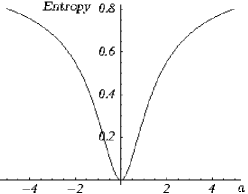
Figure 3: Entropy of the pulse as a function of the chirp $a$

We conclude this section with a remark that pulses with linear chirp are analogous to quantum mechanical wave functions of the form $\psi(x)=e^{iax^{2}}$. In the framework of quantum mechanics such wave functions belong to a wide class of the so-called contractive states kw1984b , and have been used to show the narrowing of the position uncertainty relation yuen1983 , and applied by Professor Eberly to phase entanglement kcjhe2004 . The contractive nature of the chirped pulse can be easily exhibited using an lens type $ABCD$ transformation of the chirped pulse, equivalent to the following linear transformation in time and frequency plane

$$\omega_{t}=\omega+\frac{t}{2\sigma^{2}}\,.$$ (42)

For a chirped pulse the dispersion of this observable is

$$(\Delta\omega_{t})^{2}=(\Delta\omega)^{2}+\frac{1}{4\sigma^{4}}(\Delta t)^{2}+\frac{1}{\sigma^{2}}\langle\omega t\rangle=\frac{2+a^{2}}{\sigma^{2}}-\frac{a}{2\sigma^{2}}\,.$$ (43)

For positive $a$, this formula exhibits a contraction of the uncertainty of $\omega_{t}$ similar to the narrowing of a freely evolving quantum mechanical wave packets. The narrowing is entirely due to the time-frequency correlation of the chirped pulse (34).

III.4 Time dependent spectrum for chirped pulses

In order to calculate the time-dependent spectrum for the chirped pulse, we will use for the filter response

$$\mathcal{J}(t)=\theta(t)\Gamma\sqrt{\frac{2}{\pi}}\exp\left(-\frac{t^{2}}{4\Gamma^{2}}\right)\,.$$ (44)

This function corresponds to a linear, causal and time translation invariant response of the filter. In the calculations we will assume that the observation time is larger compared with the pulse duration: $t\geq\tau_{d}$. Simple calculation shows that the spectrum is Gaussian and has the form

$$G(t,\omega)=G_{0}\exp\left(-\frac{1}{2}\mathbf{w}\,\mathbf{G}\,\mathbf{w}^{T}\right)$$ (45)

where $\mathbf{v}=(t,\omega)$ is a vector and the matrix $\mathbf{G}$ can be expressed in terms of the covariance matrices of the pulse and the filter

$$\mathbf{G}^{-1}=\mathbf{C}+\mathbf{C}_{\mathcal{J}}=\left[\begin{array}[]{cc}\Gamma^{2}+\sigma^{2}&-\frac{a}{2}\\ -\frac{a}{2}&\frac{1}{\Gamma^{2}}+\frac{1+a^{2}}{4\sigma^{2}}\\ \end{array}\right]\,.$$ (46)

The normalization constant $G_{0}$ of the time-dependent spectrum is such that

$$\int\frac{dtd\omega}{2\pi}\,G(t,\omega)=\int dt\,I(t)\,.$$ (47)

IV Linear superposition of chirped pulses

Linear superposition principle play a fundamental role in classical and quantum interference phenomena. In order to illustrate time and frequency interference we shall investigate a linear superposition of two optical pulses

$$E_{\mathrm{sup}}=E(t-t_{0})+E(t+t_{0})\,,$$ (48)

where $2t_{0}$ is a temporal separation between the pulses. This linear superposition of two electric fields of optical pulses exhibit classical interference very similar to the interference of quantum coherent states janszky1994 ; kwgh1998 .

As an example of such a superposition we take two Gaussian chirped pulses

$$E_{\mathrm{sup}}(t)=\exp\left(-\frac{(t-t_{0})^{2}}{4\sigma^{2}}(1+ia)\right)+\exp\left(-\frac{(t+t_{0})^{2}}{4\sigma^{2}}(1+ia)\right)\,.$$ (49)

The intensity of this superposition is:

$$I(t)=\exp\left(-\frac{(t-t_{0})^{2}}{2\sigma^{2}}\right)+\exp\left(-\frac{(t+t_{0})^{2}}{2\sigma^{2}}\right)+2\exp\left(-\frac{t^{2}+t_{0}^{2}}{2\sigma^{2}}\right)\cos\left(\frac{tt_{0}a}{\sigma^{2}}\right)\,.$$ (50)

The corresponding power spectrum is

$$P(\omega)=\frac{4\sigma^{2}}{\sqrt{1+a^{2}}}\exp\left(-\frac{2\omega^{2}\sigma^{2}}{1+a^{2}}\right)\cos^{2}(\omega t_{0})\,.$$ (51)

The time-frequency Wigner function of the linear superposition (49) is

$$W(t,\omega) = W_{E}(t+t_{0},\omega)+W_{E}(t-t_{0},\omega)+2W_{E}(t,\omega)\cos(2t_{0}\omega)\,.$$ (52)

In this formula the Wigner function: $W_{E}(t,\omega)$ is given by (27). From the Wigner function of the superposition it is possible to calculate time and frequency moments. Simple calculation leads to

$$\langle t^{2}\rangle=\sigma^{2}+\frac{t_{0}^{2}(1-a^{2}\exp(-\frac{t_{0}^{2}(1+a^{2})}{2\sigma^{2}}))}{1+\exp(-\frac{t_{0}^{2}(1+a^{2})}{2\sigma^{2}})}\,,$$ (53)

and

$$\langle\omega^{2}\rangle=\frac{1+a^{2}}{4\sigma^{2}}\left(1-\frac{t_{0}^{2}}{\sigma^{2}}(1+a^{2})\frac{\exp(-\frac{t_{0}^{2}(1+a^{2})}{2\sigma^{2}})}{1+\exp(-\frac{t_{0}^{2}(1+a^{2})}{2\sigma^{2}})}\right)\,.$$ (54)

From this formula we see that the spectrum of the linear superposition is reduced (squeezed) below the single pulse width. This effect is entirely due to the fact that we are dealing with a linear superposition of pulses. In Figures (4) and (5) we have depicted the Wigner function for the linear superposition with $t_{0}=4$ with no chirp and chirp $a=3$. The squeezing effect corresponding to the nonzero chirp is clearly seen.

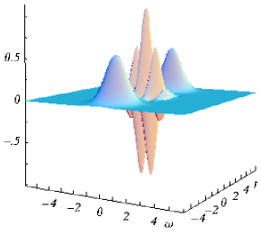
Figure 4: Plot of the Wigner function for two Gaussian pulses with no chirp $a=0$ and $t_{0}=4$.

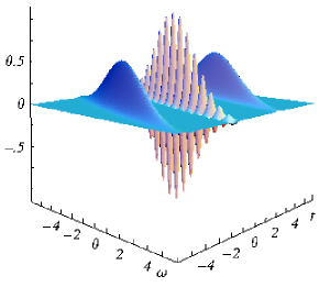
Figure 5: Plot of the Wigner function for two Gaussian pulses with chirp $a=3$ and $t_{0}=4$.

Note that in reference beck1993 , the Wigner function of a coherent two-pulse sequence with linear frequency chirp has been reconstructed experimentally using quantum tomography.

The remarkable feature of the Wigner function (52) is the fact that it contains structures in a phase space region below the Fourier uncertainty relation. In Figure (6) we have depicted the Wigner function in a space region with $\Delta\omega\leq 1/\sqrt{2}$ and $\Delta t\leq 1/\sqrt{2}$. In the framework of quantum mechanics it has been recognized that small structures on the sub-Planck scale do show up in quantum linear superpositions zurek2001 . It is clear that for linear superpositions of chirped pulses such sub-Fourier structures emerge as well. We will see in the next Section, that due to such small structures it will be possible to have pulses with zero overlap.

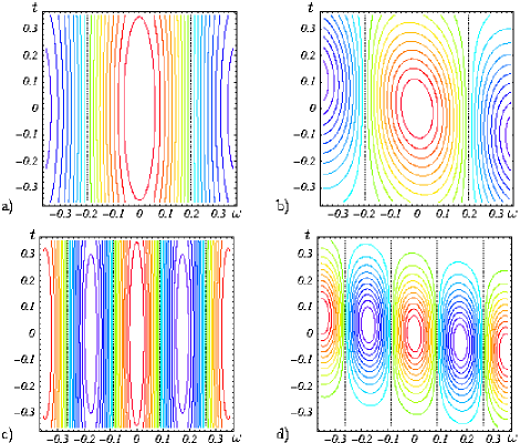
Figure 6: The interference terms of the Wigner function for two Gaussian pulses plotted at the region of the phase space below the Fourier uncertainty: a) fragment of the plot from Figure (4), i.e. $a=0$, $t_{0}=4$; b) fragment of the plot from Figure (5), i.e. $a=3$, $t_{0}=4$; c), d) similar terms obtained for larger time separation distance $t_{0}=9$ with chirps $a=0$ and $a=5$, respectively.

V Time and frequency overlap

In this Section we will investigate a FROG version (with $\mathcal{J}(t)=E^{\ast}_{\mathrm{sup}}(t)$) of the time dependent spectrum (1) applied to the linear superposition of pulses given by the formula (49)

$$G(0,\Delta)=\biggl{|}\int ds\,E^{\ast}_{\mathrm{sup}}(s)E_{\mathrm{sup}}(s)e^{i\Delta s}\biggl{|}^{2}\,.$$ (55)

Such an overlap can be easily obtained if one of the two pulses has its carrier frequency detuned by $\Delta$. In this case the FROG signal is a phase space overlap (8) of the form

$$G_{FROG}(0,\Delta)=2\pi\int dt\int d\omega\,W_{E_{\mathrm{sup}}}(t,\omega)W_{E_{\mathrm{sup}}}(t,\omega+\Delta)\,.$$ (56)

For the chirped pulses this overlap can be calculated, and as a result we obtain

$$G_{FROG}(0,\Delta)=\mathcal{N}e^{-\frac{\Delta^{2}\sigma^{2}}{2}}\left(\cos(\Delta t_{0})+e^{-\frac{t_{0}^{2}}{2\sigma^{2}}(1+a^{2})}\cosh(\Delta t_{0}a)\right)^{2}\,,$$ (57)

where $\mathcal{N}$ is a normalization constant. In Figure (7) we have depicted (57) as a function of $\Delta$, for $t_{0}=5$ and $a=5$.

Figure 7: The overlap as a function of $\Delta$ for a linear superposition with $t_{0}=5$ and $a=5$

The remarkable feature of this curve is that $G_{FROG}(0,\Delta)$ can vanish for values of $\Delta$ smaller then the frequency uncertainty in frequency. In terms of the time and frequency distribution function, the detuning $\Delta$ of the carrier frequency corresponds just to a shift of the Wigner function along the $\omega$ axis. In the case of the superposition of two Gaussian pulses, this shift affects the Gaussian peaks and the oscillating non-positive interference term. It is easy to notice that for an appropriate value of $\Delta$ this can result in a sign change of the interference term in comparison to the original function. Calculating the overlap (56) we need a product of shifted and unshifted Wigner functions. For a selected value of the shift $\Delta$, the product of the two interference terms of their Wigner functions will become negative (or zero). In Figure (8) we have depicted such a product with $t_{0}=4$ and shift $\Delta=\pi/2t_{0}$. We see that the considerably large negative contribution can cancel the positive peaks corresponding to the overlap of the non-interference terms.

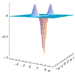
Figure 8: The product of two Wigner functions for linear superpositions of pulses with $t_{0}=4$ and $a=0$ mutually shifted in carrier frequencies by $\Delta=\frac{\pi}{2t_{0}}$.

Obviously, formula (57) can be easily obtained without using the Wigner function, but the phase-space representation (56) is especially useful to show that the sub-Fourier structures are peculiar to interference phenomena.

In quantum mechanical framework this feature is especially interesting as the zero–overlap means that the corresponding states are orthogonal, and so at a sub-Planck scale one can obtain sets of mutually orthogonal states zurek2001 . In the case of optical pulses we can obtain a similar result of pulses with zero–overlap using a shifts of frequency that are below the Fourier uncertainty relation. Certainly, the smaller is the value of this shift $\Delta$ that one wants to use, the larger $t_{0}$ has to be taken in the calculations, meaning that the Fourier/Heisenberg uncertainty relation is satisfied.

VI Conclusions

In this paper we have analyzed the connection of the time and frequency time-dependent spectrum with phase space distributions based on the Wigner and the Ambiguity functions. We have exploited the similarities between optical pulses and quantum mechanical wave packets to exhibit interference, entanglement, and sub-Fourier structures of the time and frequency phase space.

Certainly the Wigner function is not the only possible way to give a time and frequency description of optical pulses. Recently in reference lpkw2003 we have introduced a class of new phase space representations based on the so called Kirkwood–Rihaczek distribution function cohen1995 :

$$K(t,\omega)=\int\frac{ds}{2\pi}\;E^{\ast}(s)\;e^{i\omega(s-t)}\;E(t)\,.$$ (58)

Such phase space distributions provide time and frequency characteristics of optical pulses, but only phase space overlaps of these distributions have an operational meaning as a physical spectrum of light. In the case of the Kirkwood–Rihaczek function this overlap, much resembling the equation (8), is given by the following formula

$$\left|\int dtE^{\ast}_{1}(t)E_{2}(t)\right|^{2}=2\pi\int dt\int d\omega\,K_{E_{1}}(t,\omega)K^{*}_{E_{2}}{(}t,\omega)\,.$$ (59)

Thus, for the superpositions discussed in Section V, we can write the following formula

$$G_{FROG}(0,\Delta)=2\pi\int dt\int d\omega\,K_{E_{\mathrm{sup}}}(t,\omega)K^{*}_{E_{\mathrm{sup}}}(t,\omega+\Delta)\,.$$ (60)

We conclude this paper by noting that the definition of the time-dependent spectrum of light introduced 28 years ago, is still an attractive field of research producing interesting insights into the definition of the spectrum of nonstationary ensemble of optical pulses wolf2004 .

References

- (1) J. H. Eberly and K. Wódkiewicz, J. Opt. Soc. Am. 67, 1252 (1977).
- (2) See for example: S. Mallat, A Wavelet Tour of Signal Processing , (Elsevier, New York, 1999).
- (3) D. J. Kane and R. Trebino, J. Opt. Soc. Am. B 10, 1101 (1993).
- (4) K.W. Delong, R. Trebino, J. Hunter and W. E. White, J. Opt. Soc. Am. B 11, 2206 (1994).
- (5) K. H. Brenner and K. Wódkiewicz, Opt. Comm. 43, 103 (1982).
- (6) K. Wódkiewicz, Phys. Rev. Lett. 52, 1064 (1984).
- (7) See for example: C. C. Gerry and P. L. Knight, Introductory Quantum Optics, (Cambridge University Press, 2005).
- (8) C. K. Law and J. H. Eberly, Phys. Rev. Lett. 92, 127903 (2004).
- (9) W. Żurek, Nature (London) 412, 712 (2001).
- (10) E. Wigner, Phys. Rev. 40, 749 (1932).
- (11) J. Ville, Cables et Transmission 2A, 61 (1948).
- (12) W. P. Schleich, Quantum Optics in Phase Space, ((Wiley-VCH, Weinheim, 2001).
- (13) L. Cohen, Time-frequency analysis: theory and applications, (Prentice-Hall Signal Processing Series, 1995).
- (14) See for example: P. Milonni and J. H. Eberly, Lasers, (Wiley, New York, 1988).
- (15) K. Wódkiewicz, Phys. Rev. Lett. 52, 787 (1984).
- (16) H. P. Yuen, Phys. Rev. Lett. 51, 719 (1983).
- (17) K. W. Chan and J. H. Eberly, quant-ph/0404093 (2004).
- (18) J. Janszky, A. V. Vinogradov and T. Kobayashi, Phys. Rev. A 50, 1777 (1994).
- (19) K. Wódkiewicz and G. Herling , Phys. Rev. A 57, 815 (1998).
- (20) M. Beck, M. G. Raymer, I. A. Walmsley and V. Wong, Opt. Lett. 18, 2041 (1993).
- (21) L. Praxmeyer and K. Wódkiewicz, Opt. Comm. 223, 349 (2003).
- (22) S. A. Ponomarenko, G. P. Agrawal and E. Wolf, Opt. Lett. 29, 394 (2004).