Evidence of crossover phenomena in wind speed data

Abstract

In this report, a systematic analysis of hourly wind speed data obtained from three potential wind generation sites (in North Dakota) is analyzed. The power spectra of the data exhibited a power-law decay characteristic of $1/f^{\alpha}$ processes with possible long-range correlations. Conventional analysis using Hurst exponent estimators proved to be inconclusive. Subsequent analysis using detrended fluctuation analysis (DFA) revealed a crossover in the scaling exponent ($\alpha$). At short time scales, a scaling exponent of $\alpha\sim 1.4$ indicated that the data resembled Brownian noise, whereas for larger time scales the data exhibited long range correlations ($\alpha\sim 0.7$). The scaling exponents obtained were similar across the three locations. Our findings suggest the possibility of multiple scaling exponents characteristic of multifractal signals.

Keywords : long range correlations, hurst exponents, crossover phenomena, detrended fluctuation analysis, wind speed.

1 Introduction

Wind energy is a ubiquitous resource and is a promising alternative to meet the increased demand for energy in recent years. Unlike traditional power plants, wind generated power is subject to fluctuations due to the intermittent nature of wind. The irregular waxing and waning of wind can lead to significant mechanical stress on the gear boxes and result in substantial voltage swings at the terminals, [1]. Therefore, it is important to build suitable mathematical techniques to understand the temporal behavior and dynamics of wind speed for purposes of modeling, prediction, simulation and design. Attempts to identify the features of wind speed time series data were described in [2] and [3]. To our knowledge, the first paper to bring out an important feature of wind speed time series was [4]. In [4], the authors examined long term records of hourly wind speeds in Ireland and pointed out that they exhibited what is known as long memory dependence. Seasonal effects, spatial correlations and temporal dependencies were incorporated to build suitable estimators. Trends in long term wind speed records were also suggested in [5]. However, in [4], short memory temporal correlations were suggested by an examination of the autocorrelation function. Evidence for the presence of long memory correlations was provided by inspecting the periodogram of the residuals from a fitted and autoregressive model of order nine i.e. AR(9), [4].

In this paper, we provide a systematic method to identify, more importantly quantify the index of long range correlations in wind speed time series data. We make use of a fairly robust and powerful technique called Detrended Fluctuation Analysis (DFA) in our analysis, [25]. The rest of this paper is organized as follows. In Sec.2, the acquisition of wind speed data is described. In Sec.3, traditional analysis of the hourly wind speed using power spectral techniques and Hurst estimators is discussed along with some of their limitations. Detrended fluctuation analysis (DFA) is used to capture the crossover phenomena in wind speed. Finally, the conclusions are summarized in Sec. 4.

2 Data Acquisition

In this section, we provide a brief description of the wind speed data acquisition system. The wind speeds at three different wind monitoring stations in North Dakota are recorded by means of conventional cup type anemometers located at a height of 20 m. Wind speeds acquired every two seconds are averaged over a 10 minute interval to compute the 10 minute average wind speed. The 10 minute average wind speeds are further averaged over a period of one hour to obtain the hourly average wind speed. In this procedure, the computed hourly average wind speed is simply equivalent to averaging the observations every two seconds for one hour. The hourly average wind speeds are preferred over the 10 minute speeds to minimize storage requirements for several years of data. The site details of the monitoring stations are provided in Table 1. In our analysis, we consider a period from 11/29/2001 to 03/28/2003 for the wind speed records. Fig.1 shows the wind speed ($v$ in $m/s$) variability at the three locations. The aim of the present study is to characterize and quantify the apparently irregular fluctuations of the wind speed in Fig.1. In the following section, the analysis of wind speed data using three different techniques is provided.

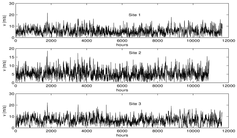
Figure 1: Wind speed variations at the three locations.

Station	Latitude	Longitude	Elevation (ft)
Site 1	N 47 27.84’	W 99 8.18’	1570
Site 2	N 46 13.03’	W 97 15.10’	1070
Site 3	N 48 52.75’	W 103 28.44’	2270

Table 1: Station Locations

3 Analysis of wind speed data

3.1 Spectral Analysis

The power spectrum $S(f)$ shown in Fig. 2 exhibits a power-law decay of the form $S(f)\sim 1/f^{\beta}$. The auto-correlation functions (ACF) decay slowly to zero and the first zero crossing of the ACFs occur at lags of 61, 56 and 60 hours respectively for the three data sets. Such features are characteristic of statistically self-similar processes with well defined long range power-law correlations, [9]. In a broad sense, long range correlations indicate that samples of the time series that are very distant in time are correlated with each other and can be captured by the auto correlation function or equivalently, the power spectrum (as in Fig. 2) in the frequency domain. More precisely, a time series is self similar if

$$y(t)\equiv a^{\alpha}y(t/a)$$ (1)

where $\equiv$ in Eqn. (1) is used to denote that both sides of the equation have identical statistical properties. The exponent $\alpha$ in Eqn. (1) is called the self-similarity parameter, or the scaling exponent. We note that while classical tools such as autocorrelation functions, and spectral analysis can give preliminary indications for the presence of long range correlations, it may be difficult to use them unambiguously to determine the scaling exponent. Additionally, these methods are susceptible to non-stationary effects such as trends in the data which are commonly encountered. It is thus important to seek alternative measures that are potentially better suited than classical tools to capture signal variability under different temporal scales. In the following section, a few certain standard methods in estimating long range correlations along with their limitations is discussed.

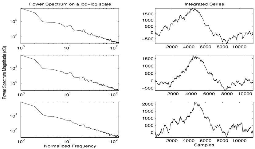
Figure 2: On the left is the power spectrum of the wind data obtained at the three locations, Site 1 (top) , Site 2(middle) and Site 3 (bottom) respectively. The corresponding integrated series is shown on the right.

3.2 Hurst Exponents

Hurst exponents have been successfully used to quantify long range correlations in plasma turbulence [11], [12], finance [13] [14], network traffic, [15] and physiology, [16]. Long range correlations are said to exist if $1/2<H<1$ (see [17], [18] for details). There are several methods for the estimation of the Hurst exponent such as variance method, re-scaled range (R/S), analysis, periodogram method, Whittle estimator and wavelet based methods. Table 1 shows the Hurst exponents estimated by various methods using SELFIS, [19] a tool for the analysis of self-similar data for all the three data sets. For the Whittle and Abry-Veicht methods, $`int^{\prime}$ refers to the 95 % confidence intervals in Table 2. In the case of variance method, re-scaled range (R/S) and Absolute moments, $c$ refers to the correlation coefficient in %.

3.2.1 Limitations of traditional Hurst estimators

We note from Table 1 that, for a given method, the Hurst exponent estimation is consistent across the three different data sets. However, for a given data set, we note that there is no consistency in the estimation of the exponents across the different methods. While the Variance, R/S and Absolute moments methods yield Hurst exponent estimates in the range (0.6-0.8), the Whittle and Abry-Veicht methods yield exponents close to 1 and 1.4 respectively. The discrepancy in the results indicate potential difficulties on applying Hurst estimators to experimental data obtained from physical processes. Some of the estimators implicitly assume stationarity of the data and can hence they could be susceptible to nonstationarities, [20]. Each of the Hurst estimators are derived under certain assumptions (see [21], [17] for details), and while they can yield consistent estimates for synthetic data, there could be discrepancies in the case of experimental data with trends. For example, the R/S method, by the very nature of its construction cannot be used to detect an exponent greater than one that may be present in the data, [23]. The Whittle estimator (a parametric method based on the maximum likelihood estimator) implicitly assumes that the parametric form of the spectral density, or equivalently, the auto-correlation function is known. An inappropriate choice of the parametric form could result in potentially biased estimations, [24]. Some of the subtleties involved in traditional estimators can be also found in [12]. An additional problem arises if the given process contains multiple scaling exponents under different scaling regions in which case, Hurst exponent estimators are difficult to apply directly. When multiple scaling exponents are present, linear regression cannot be used to compute the exponent over all scales and such an attempt can have adverse effects on the Hurst exponent estimate as the regression may capture the exponent over a certain scale. To summarize, the conflicting estimates produced by these estimators indicates that one cannot in general, use a “blind” black-box approach when dealing with processes with long range correlations.

It has also been pointed out that long-range correlations can manifest themselves as slow moving non-stationary trends, such as seasonal cycles, [29]. Thus traditional techniques such as spectral analysis and Hurst estimators have their limitations. These techniques are also not well suited to provide insight in to possible change in the scaling indices (crossover, Sec 3.3). Thus it is important to explore the choice of alternate measures to quantify the scaling exponent from the given data. In the following section, we shall present an over view of such a method, i.e. Detrended Fluctuation Analysis (DFA).

3.3 Detrended Fluctuation Analysis (DFA)

The DFA first proposed in [25] is a powerful technique and has been successfully used to determine possible long-range correlations data sets obtained from diverse settings [26], [27], [28], [29]. A brief description of DFA is included here for completeness. A detailed explanation can be found in elsewhere, [25]. Consider a time series $\{x_{k}\},k=1,\dots N$. Then, the DFA algorithm consists of the following steps.

• Step 1 The series $\{x_{k}\}$ is integrated to form the integrated series $\{y_{k}\}$ given by

  $$y(k)=\sum_{i=1}^{i=k}[x(i)-\bar{x}]\;\;\;k=1,\dots N$$ (2)

• Step 2 The series $\{y_{k}\}$ is divided in to $n_{s}$ non-overlapping boxes of equal length $s$, where $n_{s}=int(N/s)$. To accommodate the fact that some of the data points may be left out, the procedure is repeated from the other end of the data set and $2n_{s}$ boxes are obtained, [25].

• Step 3 In each of the boxes, the local trend is calculated by a least-square fit of the series and the variance $F^{2}(v,s)$ is calculated from

  $$F^{2}(v,s)=\{\frac{1}{s}\sum_{i=1}^{i=s}\{y[(v-1)s+i]-y_{v}(i)\}^{2}$$ (3)

  for each box $v=1,\dots n_{s}$. Similarly, the computation is done for each box $v=n_{s}+1,\dots 2n_{s}$ by

  $$F^{2}(v,s)=\{\frac{1}{s}\sum_{i=1}^{i=s}\{y[N-(v-n_{s})s+i]-y_{v}(i)\}^{2}$$ (4)

  where $y_{v}$ is the fitting polynomial in box $v$. Depending on the polynomial, i.e. linear, quadratic, cubic, quartic, the procedure is called DFA1, DFA2, DFA3 and DFA4 respectively. The second order fluctuation is calculated by averaging the variations over each of the boxes , i.e.

  $$F_{2}(s)=\{\frac{1}{2n_{s}}\sum_{v=1}^{v=2n_{s}}[F^{2}(v,s)]\}^{1/2}$$ (5)

• Step 4 The computation in Step 3 is repeated over various time scales by varying the box size $s$. A log-log graph of the fluctuations $F_{2}(s)$ versus $s$ is calculated . Linear relationships in the graph indicate self-similarity and the slope of the line $F_{2}(s)$ vs $s$ on the log-log plot determines the scaling exponent $\alpha$.
  

The value of $\alpha$ obtained from the DFA algorithm quantifies the nature of correlations. Values of $\alpha$ in the range (0, 0.5) characterize anti-correlations (large fluctuations are likely to be followed by small fluctuations and vice-versa) and values of $\alpha$ in the range (0.5,1) characterize persistent long range correlations (large/small fluctuations are likely to be followed by large/small fluctuations in that order) with $\alpha=0.5$ representing uncorrelated (white) noise. If $\alpha>1$, correlations exist, but they are no longer of a power law form, [29]. For exactly self-similar processes, the exponent ($\beta)$ from the power spectrum ($S(f)\sim 1/f^{\beta})$ is related to the DFA exponent $\alpha$ by $\beta=2\alpha-1$, [17]. For example, $\alpha=0.5$ is equivalent to $\beta=0$ which characterizes white noise, while $\alpha=1$ is equivalent to $\beta=1$ which corresponds to $1/f$ noise and $\alpha=1.5$ which corresponds to $\beta=2$ characterizes Brown noise, the integration of white noise. However in the case of experimental data which may be subject to trends and non-stationarities, an unambiguous determination of scaling exponents from the power spectrum may be difficult, [30]. DFA minimizes trends by local de-trending (Step 3) and hence it is robust to trivial non-stationarities. While the original DFA [25], used only differencing of the integrated series, Fig. 1, recent reports have pointed out that a choice of higher order polynomial detrending can avoid spurious results [31], [32]. Polynomial trends are minimized by local detrending (Step 3). This renders DFA to be robust to non-stationarities contributed by polynomial trends and prevents spurious detection of long-range correlations which is an outcome of such trends. The scaling exponents are estimated by linear regression of the log-log fluctuation curve, [25]. However, this can lead to spurious results when there is more than one scaling exponent which is true in the case of crossover phenomena, [25]. A crossover usually arises due to changes in the correlation properties of the signal at different temporal or spatial scales (see Figs. 3, 4 and 5), [32]. Therefore, extracting the global exponent can be misleading, especially in the presence of crossover phenomena [29], [27]. Recent studies have suggested comparing the results obtained on the original to constrained randomized shuffles of the given data [29]. Unlike traditional bootstrap realizations, constrained randomized shuffles (surrogates) are obtained by resampling the given data without replacement. In surrogate testing, one generates what are termed as “constrained realizations”, [6], [7]. The constraint here is on retaining the distribution of the original data in the surrogate realization. While the temporal structure is destroyed, the distribution of the original data is retained in the surrogate realization. The null hypothesis addressed by the random shuffled surrogates (which retain the pdf of the original data) is that the original data is “uncorrelated”. The choice of the random shuffled surrogates helps us to reject the claim that the observed scaling exponent is due to the distribution as opposed to the correlation in the given data. Comparison of the scaling exponents obtained on the original data to that of the random shuffled surrogates is encouraged by earlier reports [32], [8], [26], [22], [23]. A good exposition on the concepts of surrogate analysis can be found in [6], [7], [33].

While the DFA has been shown to be a robust algorithm compared to traditional Hurst exponent estimators in the presence of non-stationarities, there are a few subtleties in the application and interpretation of the results obtained from DFA. A common problem with DFA is that crossovers can occur due to a genuine change in the correlation properties of the signal, or due to trends. While a choice of higher order polynomial de-trendings can eliminate polynomial trends and avoid spurious results [31], [32], the presence of strong sinusoidal trends can induce spurious crossovers, [32] (a detailed discussion of this issue is reported in [32]). Since trends are unavoidable in time series generated by physical processes, it may be prudent to first recognize their presence before applying DFA. For the data sets considered in this study we did not observe strong sinusoidal trends and therefore pursued the application of DFA, the results of which are described in the next section.

3.4 Results with DFA

The log-log plot of the fluctuation $F(s)$ versus the time scale $(s)$, for the three data sets and their surrogates (indicated by the dotted lines) with different order polynomial detrending (indexed by 1,2,3,4) are shown in Figs 3, 4 and 5. The scaling exponents estimated by linear regression for all four orders of detrending on the original data and its surrogates are summarized in Table 3.

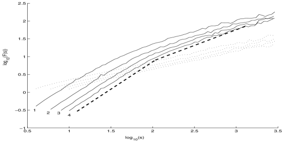
Figure 3: log-log plot of the fluctuation functions of the original data and its random shuffled surrogate (dotted lines) for Site 1. The order of polynomial detrending $d$ (1,2,3,4) for the original data set is indicated. The fourth order ($d=4$) detrending on the original data is shown by the dashed bold line.

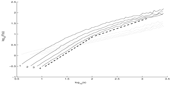
Figure 4: log-log plot of the fluctuation functions of the original data and its random shuffled surrogate (dotted lines) for Site 2. The order of polynomial detrending $d$ (1,2,3,4) for the original data set is indicated. The fourth order ($d=4$) detrending on the original data is shown by the dashed bold line.

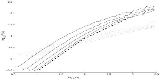
Figure 5: log-log plot of the fluctuation functions of the original data and its random shuffled surrogate (dotted lines) for Site 3. The order of polynomial detrending $d$ (1,2,3,4) for the original data set is indicated. The fourth order ($d=4$) detrending on the original data is shown by the dashed bold line.

DATA	Variance		R/S		Abs. Moments		Whittle		Abry-Veicht		Period
	$H$	$c$	$H$	$c$	$H$	$c$	$H$	$int$	$H$	$int$	$H$
Site 1	0.778	96.73	0.595	97.36	0.726	94.4	0.99	0.98-1.01	1.36	1.34-1.38	1.028
Site 2	0.772	97.3	0.608	97.35	0.712	95.5	0.99	0.98-1.02	1.33	1.31-1.35	1.059
Site 3	0.721	95.7	0.593	96.65	0.654	95.8	0.99	0.98-1.02	1.36	1.34-1.37	1.077

Table 2: Hurst exponent estimation by various methods

DATA	d=4		d=3		d=2		d=1
	$\alpha$	$\alpha^{*}$	$\alpha$	$\alpha^{*}$	$\alpha$	$\alpha^{*}$	$\alpha$	$\alpha^{*}$
Site 1	1.03	0.51	0.99	0.51	0.94	0.51	0.85	0.51
Site 2	1.01	0.52	0.96	0.52	0.92	0.52	0.83	0.52
Site 3	1.06	0.49	1.02	0.49	0.97	0.48	0.88	0.48

Table 3: Global scaling exponent of the original data ($\alpha)$ and it surrogates ($\alpha^{*}$)

DATA	d=4		d=3		d=2		d=1
	$\alpha_{1}$	$\alpha_{2}$	$\alpha_{1}$	$\alpha_{2}$	$\alpha_{1}$	$\alpha_{2}$	$\alpha_{1}$	$\alpha_{2}$
Site 1	1.47	0.75	1.45	0.70	1.38	0.66	1.23	0.59
Site 2	1.44	0.70	1.40	0.65	1.35	0.62	1.20	0.58
Site 3	1.44	0.77	1.42	0.71	1.38	0.67	1.26	0.60

Table 4: Local scaling exponents of the original data ($\alpha_{1})$ and ($\alpha_{2}$)

From Table 3, we note that the choice of linear detrending (DFA1, i.e. $d=1$) yields estimates of $\alpha\sim 0.85$ consistently at all three locations. Whereas, higher order detrendings ($d=2,3,4$) indicate an exponent $\alpha\sim 1$ consistently at all three locations which suggests a possible $1/f$ type behavior. For the surrogate data sets ($a^{*}$) in Table 3, we note that all four choices of detrending yield exponents very close to $0.5$ at all three locations which shows that scaling in the original data is an outcome of the correlations present in it and not due to its distribution.

We further note from Figs. 3, 4 and 5 that unlike the surrogates, the log-log plot of the original data sets at all three locations is not linear. For low orders of detrending $d=1,2,3$, the slope of the fluctuation functions of the original data set gradually changes as seen in Figs 3, 4 and 5. However, for $d=4$ (fourth order detrending), the transition of slope is comparatively abrupt in the fluctuation function around $s_{\times}\sim 10^{2}$ which suggests the existence of more than one scaling exponent. In this case, the global scaling exponent shown in Table 3 is insufficient to capture the change in scaling exponent. Therefore, the scaling region is partitioned in to two regions around $s=s_{\times}$. In the region $s<s_{\times}$, the slope of the fluctuation function is given by $\alpha_{1}$ and in the region $s>s_{\times}$, the slope is given by $\alpha_{2}$. These represent what we call “local scaling exponents”. Thus, the “crossover” from one scaling exponent ($\alpha_{1}$) to the other ($\alpha_{2}$) is seen to occur at approximately at a time scale $s_{\times}\sim 10^{2}=100$ hours. The local scaling exponents $(\alpha_{1},\alpha_{2})$ estimated by DFA for these two regions, using different order polynomial detrending for the three data sets are summarized in Table 4. As a comment, we would like to mention that such intricacies are not evident from the power spectrum, Fig. 2 and Hurst analysis (Sec 3.2).

Recall from Sec. 3.2 that while some of the methods (Variance method, R/S and Absolute moments) yielded exponent estimates in the range (0.6-0.8), the Abry-Veicht method produced an estimate close to 1.4. On the other hand, DFA in addition to identifying the exponents also helps in demarcating the regions (time scales in the signal) where these exponents are contained.

From Table 4, we note that DFA1 yields an exponent $\alpha_{1}$ close to 1.2 whereas DFA2,3,4 yield exponents close to 1.45 at all three locations. For the exponent $\alpha_{2}$, we note that while DFA1 yields estimates close to 0.6, DFA2,3,4 yield exponents close to 0.7. Therefore, it is reasonable to say that the original signal possesses at least two scaling exponents over two time scales. At short time scales ($s<100$ hours), the data exhibits behavior similar to Brown noise $(\alpha\sim 1.45)$, whereas for longer time scales $(s>>100$ hours) one observes persistent long-range correlations $(\alpha\sim 0.70)$. Interestingly, the results obtained across the data obtained from different geographical locations seem to exhibit a similar behavior.

4 Conclusions

Long term records of hourly average wind speeds at three different wind monitoring stations in North Dakota are examined. Preliminary spectral analysis of the data indicates that wind speed time series contain long range power-law correlations. Analysis using Hurst estimators were inconclusive. A detailed examination using DFA indicated a crossover and revealed the existence of at least two distinct scaling exponents over two time scales. While the data resembled Brownian noise over short time scales, persistent long range correlations were identified over longer time scales. The scaling behavior was consistent across the three locations and were verified using different orders of polynomial trending. It is interesting to note that despite the inherent heterogeneity across spatially separated locations, certain quantitative features of the wind speed are retained. While several factors including friction, topography and surface heating are known to contribute towards wind speed variability, the present report seems to indicate that the combined effect of these factors may themselves be subject to variability over different time scales. A possible explanation for the crossover may be that on short time scales (tens of hours), the fluctuations in wind speed may be dominated by atmospheric phenomena governed by the “local or regional” weather system whereas on longer time scales (extending from several days to months), the fluctuations may be influenced by more general “global” weather patterns. While the present study indicates two distinct scaling exponents, a closer inspection of longer records of wind speed at finer resolutions may possibly reveal a spectrum of scaling exponents characteristic of multifractals. However, this is more of a conjecture at this point. We plan to investigate this in greater detail in subsequent studies.

References

- [1] Peter Fariley, “Steady As She Blows”, IEEE Spectrum, vol. 12, no. 1, pp. 35-39, Aug 2003.
- [2] J. Haslett and E. Kelledy, “The assessment of actual wind power availability in Ireland”, Env Res, 3, 333-348, 1979.
- [3] A. E. Raftery, J. Haslett and E. McColl, “Wind power : a space time process ?”, Time Series Analysis : Theory and Practice 2, ed. O. D. Anderson, pp. 191-202, 1982.
- [4] J. Haslett and A. E. Raftery, “Space-time Modelling with Long-memory Dependence : Assessing Ireland’s Wind Power Resource (with discussion) ”, Appl. Statistics, vol. 38, no. 1, pp. 1-50, 1989.
- [5] J. P. Palutikof, X. Guo and J. A. Halliday, “The reconstruction of long wind speed records in the UK ”, In: Wind Energy Conversion 1991 (Eds. D.C. Quarton and V.C. Fenton), pp.275-280 Mechanical Engineering Publications, London.
- [6] J. Theiler, S. Eubank, A. Longtin, B. Galdrikian, and J. D. Farmer, “Testing for nonlinearity in time series: The method of surrogate data”, Physica D 58, 77 (1992).
- [7] T. Schreiber and A. Schmitz, “Improved surrogate data for nonlinearity tests”, Phys. Rev. Lett. 77, 635 (1996), chao-dyn/9909041.
- [8] A. L. Goldberger, L. N. Amaral, J. Hausdorff, P. Ch. Ivanov, C. K. Pend and H. E. Stanley, “ Fractal Dyanamics in Physiology : Alterations with disease and aging”, Proc. National Acad. Sci., vol. 19, suppl.1, Feb 19, 2002, pp : 2466-2472.
- [9] J. Feder, Fractals, Plenum Press, New Yok, 1988.
- [10] H. E. Hurst, “Long-term storage capacity of reservoirs”, Trans. Amer. Soc. Civ. Engrs., vol.116, pp. 770-808, 1951.
- [11] Yu CX, Gilmore M, Peebles WA and Rhodes TL, “Structure Function Analysis of Long-Range Correlations in Plasma Turbulence”, Phy. of Plasmas vol.10, pp : 2772-2779, 2003.
- [12] Gilmore M, Yu CX , Rhodes TL and Peebles WA, “Investigation of rescaled analysis, Hurst exponent and long term correlations in plasma turbulence in Plasma Turbulence”, vol.9, no. 4, pp : 1312 - 1317, 2002.
- [13] J. Moody and L. Wu, “Long memory and Hurst exponents of tick-by-tick interbank foreign exchange rates”, Proceedings of Computational Intelligence in Financial Engineering, IEEE Press, Piscataway, NJ, pp. 26-30, 1995.
- [14] R. Weron and B. Przybylowicz, ”Hurst Analysis of Electricity Price Dynamics”, Physica A, vol.283, pp. 462-468, 2000.
- [15] A. Erramilli, M. Roughan, D. Veitch, and W. Willinger, “Self-similar traffic and network dynamics”, Proceeding of the IEEE, vol.90,(5), pp. 800-819, May 2002.
- [16] P. Ch. Ivanov, L. Amaral, A. Goldberger, S. Havlin, M. G. Rosenblum, Z. R. Struzik and H. E. Stanley, “Multifractality in human heartbeat dynamics”, Nature, vol. 399, vo.3, pp. 461-465, June 1999.
- [17] J. Beran, “Statistics for Long Memory Processes”, Chapman and Hall, NewYork, 1994.
- [18] J. B. Bassingthwaighte, L. S. Liebovitch and B. J. West, Fractal phyysiology, Americal Physiological Society, Oxford, pp. 78-89, 1994
- [19] T. Karagiannis, M. Faloutsos and M. Molle, “A User-Friendly Self-Similarity Analysis Tool”, ACM SIGCOMM Computer Communication Review, 2003. (available from http://www.cs.ucr.edu/ tkarag/Selfis/Selfis.html)
- [20] P. Abry and D. Veitch, “Wavelet Analysis of Long-Range-Dependent Traffic”, IEEE Trans. on Information Theory, vol.44,no.1,pp : 2-15, January 1998.
- [21] M. S. Taqqu, V. T. Teverovsky and W. Willinger, “Estimators for long range dependence: An empirical study”, Fractals, vol. 3, no. 4 pp: 785-798, 1995.
- [22] K. Matia, Y. Ashkenazy and H. E. Stanley, “ Multifractal properties of price fluctuations of stocks and commodities”, Europhysics Letters, vol. 61 (3), pp : 422-428, 2003.
- [23] E. K. Bunde, J. W. Kantelhardt, P. Braun, A. Bunde, and S. Havlin “Long term persistence and multifractality of river runoff records : Detrended fluctuation studies”, arXiv:physics/0305078 v2 30 Oct 2003.
- [24] B. Audit, E. Bacry, J.F. Muzy and A. Arneodo, “Wavelets based estimators of scaling behavior” IEEE, Trans. on Information Theory vol. 48, 11 pp 2938-2954, 2002.
- [25] C. K. Peng, S. V. Buldyrev, S. Havlin, M. Simons, H. E. Stanley and A. L. Goldberger, ”Mosaic organization of DNA nucleotides, Phys. Rev. E, vol. 49, pp. 1685-1689, 1994.
- [26] J. M. Hausdorff, C. K. Peng, Z. Ladin, J. Y. Wei and A. L. Goldberger, “Is walking a random walk ? Evidence for long range correlations in stride interval of human gait”, Journal of App. Physiology, vol. 78, pp. 349-358, 1995.
- [27] N. Vandewalle and M. Ausloos, “ Coherent and random sequences in financial fluctuations”, Physica A, vol. 246, pp. 454-459, 1997.
- [28] K. Ivanova and M. Ausloos, “Application of Detrended Fluctuation Analysis (DFA) method for describing cloud breaking”, Physica A, 274, pp. 349-354, 1999.
- [29] C. K. Peng, S. Havlin, H. E. Stanley and A. L. Goldberger, “Quantification of scaling exponents and crossover phenomena in nonstationary heartbeat time series”, Chaos, vol. 5, pp. 82-87, 1995.
- [30] E. K. Bunde, A. Bunde, S. Havlin, H. E. Roman, Y. Goldreich and H. J. Schellnhuber, “Indication of a Universal Persistence Law Governing Atmospheric Variability”, Physical Review Letters, vol. 81, no.3, pp : 729 - 732, July 1998.
- [31] A. Bunde, S. Havlin, J. W. Kantelhardt, T. Penzel, J. H. Peter and K. Voigt, “Correlated and Uncorrelated Regions in Heart rate fluctutions during sleep”, Phy. Rev. Lett., vol. 85, no. 17, pp. 3736-3739, 2000.
- [32] K. Hu, P. Ivanov, Z. Chen, P. Carpena and H. E. Stanley, “Effects of trends on detrended fluctuation analysis”, Phy. Rev. E, vol. 64, 011114, 2001.
- [33] M. Small and C. K. Tse, “Detecting Determinism in Time Series : The method of Surrogate Data”, IEEE Trans. on Circuits and Systems-I Fundamental Theory and Applications, vol. 50, no. 3, pp. 663-672, May 2003.
- [34] W. H. Press, “Flicker noise in astronomy and elsewhere”, Comments Astrophys, vol. 7, pp. 103-119, 1978.