The Robin Hood method - a novel numerical method for electrostatic problems based on a non-local charge transfer

Abstract

We introduce a novel numerical method, named the Robin Hood method, of solving electrostatic problems. The approach of the method is closest to the boundary element methods, although significant conceptual differences exist with respect to this class of methods. The method achieves equipotentiality of conducting surfaces by iterative non-local charge transfer. For each of the conducting surfaces non-local charge transfers are performed between surface elements which differ the most from the targeted equipotentiality of the surface. The method is tested against analytical solutions and its wide range of application is demonstrated. The method has appealing technical characteristics. For the problem with $N$ surface elements, the computational complexity of the method essentially scales with $N^{\alpha}$, where $\alpha<2$, the required computer memory scales with $N$, while the error of the potential decreases exponentially with the number of iterations for many orders of magnitude of the error, without the presence of the Critical Slowing Down. The Robin Hood method has a large potential of application in other classical as well as quantum problems. Some possible applications outside electrostatics are outlined.

, and

1 Introduction

The methods of solving electrostatic problems today range from the fundamentals of classical physics [1, 2, 3, 4], practically representing the scientific heritage, to the state-of-the-art computational approaches [5, 6, 7, 8] widely used for handling complex technological problems. The development of computational power in the last decades has resulted in a large number of available efficient methods for the solution of potential problems in electrostatics, as well as in other areas of physical, engineering and technological applications. According to the basic approach towards the main goal of electrostatic problems, the determination of the electric potential in the relevant segment of space, methods can be roughly divided into Finite Element Methods (FEM), Boundary Element Methods (BEM) and Finite Difference (FD) computational methods [9, 10]. In very general terms, FEM and BEM solve for the charge distribution at relevant objects (or their boundaries) and thus obtain the potential indirectly, whereas FD methods determine the potential directly in the relevant segment of space.

In this paper we develop a robust new method for solving large classes of electrostatic problems. The usefulness and applicability of the method with respect to other potential problems will also be outlined.

“As simple as it gets”. In this paragraph we give a clear overview of the simple physical idea that has guided us towards the development of the method presented here. Owing to the abundance of technical details given later, the main idea could be blurred and that simple idea is what gives our method efficiency and robustness. To give the insight into the core of the method, we describe a simple problem. Suppose that we have an ideal, insulated and charge neutral, metal sphere standing in vacuum and we bring a point charge next to it. What will happen with the charge distribution on the sphere? It will redistribute until all the surface of the sphere becomes equipotential. That is the stationary situation: the charge will not redistribute any further because the potential is the same everywhere on the sphere surface. That is a very simple high-school argument which reveals the qualitative nature of the stationary solution. With equal simplicity, one can deduce that the electric field must be perpendicular to the surface of the metal, as indeed will be seen in the examples treated in this paper. Following only this equipotentiality principle, we employ a straightforward numerical procedure to find a complete quantitative solution of this electrostatic problem. First, we divide a sphere into finite triangle elements, each having some surface charge. The initial surface charge distribution is chosen in such a way to respect the charge neutrality of the sphere. One can simply set the charge distribution to zero on the entire sphere. We calculate the electrical potential at each of these elements due to charges on all triangles and a point charge. We determine two of the triangles which have the highest and the lowest potential, respectively, and transfer the charge from one of these two selected elements to the other in such a manner that after the transfer the potentials on these two elements are exactly the same. Since we do only the charge transfer, the total charge on the sphere remains conserved, i.e. the sphere remains neutral. Then the update of the potential, resulting from the charge transfer, is performed. We iterate this process. The main idea is that such a procedure will lead to a more and more equipotential surface, and eventually converge to the solution of the electrostatic problem. Since the main idea of the method, namely taking from the maximum and giving to the minimum thus making them equal, to the principal ideas of Robin Hood (RH), we suggest this name for out method.

The conceptual importance of this “as simple as it gets” reflection is the reason for placing this brief description of the method already here in the introduction. All properties of the RH method stem from this main simple idea of min-max equipotentialization and not from the particular implementation. As a matter of fact, all essential elements of the RH method are provided in the description given above, which best illustrates the conceptual attractiveness of the RH method. The rest of the paper is devoted to the elaboration of the stated principles and the description of the elements of implementation of the RH method which raise afore-mentioned simple ideas to the level of a powerful calculational technique.

The paper is organized as follows: The second section is devoted to the physical foundations of the RH method. This section gives general elements of the method as well as the specific features for the cases of insulated conducting surfaces and conducting surfaces at the exterior potential. The third section specifies details of the implementation of the method. The fourth section comprises several examples, some of which show the reliability of the RH method by comparison with analytical solutions, while others demonstrate the broad applicability of the method. The fifth section exposes the technical characteristics, like the computational complexity, memory requirements, speed of convergence and others. The sixth section outlines the possibilities of extension of the RH method beyond electrostatics. The seventh section closes the paper with conclusions.

2 Physical foundations

A large class of electric field configurations is achieved by an appropriate spatial configuration of various conductors. These conductors, such as electrodes, cables, plates, etc. are either maintained at the potentials of exterior voltage sources or are insulated. For static electric fields, there are no electric currents and all parts of every conductor are at the same potential. The principle of equipotentiality of conductors in electrostatics is at the very core of the computational method presented in this paper.

Despite the fact that here we principally consider the electrostatic case, it is instructive to take a look into the process of attaining the static configuration of the electric field. When one of the conductors is attached to an exterior voltage source or charges are deposited close to the surfaces of the conductors, the electric currents flow and rearrange the distribution of free charges in the conductors until the surfaces of the conductors become equipotential again. Therefore, every static configuration of the electric field is initially achieved by the redistribution of the free charge in the conductors. The description of the process of reaching some electrostatic configuration is generally more complex than the description of the electrostatic configuration itself. However, it is tempting to investigate the usefulness of the concept of the charge redistribution in determining the electrostatic configurations themselves. Here we present the method of solving electrostatic problems using the iterative redistribution of the charge at the surfaces of conductors.

We consider the general problem of determining the electric potential in the spatial segment delimited by conducting surfaces. The underlying assumption of the method is that the Green function of the system is known, i.e. that with the knowledge of the charge distribution at all surfaces it is possible to determine the electric potential at any point of interest. This assumption represents the most fundamental limitation of the method, but is, on the other hand, justified for a very large class of both theoretically and practically interesting problems. The conducting surfaces either are kept at defined potentials or are insulated. Every conducting surface is divided into surface elements and a point is chosen within each surface element. The potential is calculated in the chosen point and in the remainder of the text this point will be referred to as the point of calculation (POC). The area of the surface element $i$ is denoted by $\Delta S_{i}$, the coordinates of its POC by $\vec{x_{i}}$ and the potential at its POC by $U_{i}$. In the practical implementation of the method, described in section 3, the surfaces are divided into triangles and the POCs are the barycentres of the triangles. This choice is motivated by the fact that the dipole of the uniformly charged triangle vanishes when it is calculated in the reference frame centered at its barycentre. This feature will be exploited in the implementation of the RH method. The aim of the method is to achieve the equipotentiality of each of the conducting surfaces. Practically, this is realized by achieving the equality of the potential at all POCs for every individual conducting surface, to a predefined accuracy. In the case of conducting surfaces kept at a fixed potential, the potential achieved at POCs is the potential of the exterior voltage source, while for the insulated conducting surfaces, the achieved potential is obtained as one of the results of the method. It is assumed that the surface charge density is constant within every surface element. The surface charge density of the surface element $i$ is $\sigma_{i}$, while its charge is $q_{i}=\sigma_{i}\Delta S_{i}$.

In the process of finding the static distribution of the charge at the conducting surfaces, we start from some initial distribution of the charge at each of the conducting surfaces. Using the known Green function, it possible to calculate the potential at each POC coming from the entire charge distribution in the system:

$$U(\vec{x})=\int_{\partial V}G(\vec{x},\vec{x^{\prime}})\sigma(\vec{x^{\prime}})\,dS^{\prime}\;,$$ (1)

with the Green function $G(\vec{x},\vec{x^{\prime}})=k\mid\vec{x}-\vec{x^{\prime}}\mid^{-1}$ and $\partial V$ stands for all boundary surfaces of the system. In our method, the analytic expression (1) can be cast into the discretized form

$$U_{i}=\sum_{j}I_{ij}q_{j}\;,$$ (2)

where

$$I_{ij}=\frac{1}{\Delta S_{j}}\int_{\Delta S_{j}}k\mid\vec{x_{i}}-\vec{x^{\prime}}\mid^{-1}\;dS^{\prime}\,.$$ (3)

In the calculation of the potential at a given POC one needs to compute the contributions of all surface elements, including the contribution from the surface element within which the POC is situated. Once the potential at all POCs is known, we can find a pair of POCs at which potential differs the most from the target value. Finally, charge transfers to/from chosen surface elements (where POCs from the chosen pair are situated) are performed in order to equalize the potentials at the POCs of the chosen pair. The procedure of equalizing potential differs somewhat, depending on whether the conducting surface is kept at the exterior potential or is insulated. Therefore we describe this procedure separately for each of the two cases.

Insulated conducting surface. In this case, there is no target potential which needs to be achieved in the process of determining the static surface charge distribution. The only condition that must be satisfied is the equipotentiality of the surface. Therefore, we choose two points which differ the most from the targeted equipotential configuration: the POC of the maximal potential and the POC of the minimal potential at the surface. We denote the POCs of the maximal and the minimal potential by $m$ and $n$, respectively. The potentials of the two chosen POCs are equalized by the charge transfer from the point of the maximal potential to the point of the minimal potential. If the amount of charge $q$ is transferred from $m$ to $n$, the potentials at these two points after the transfer will be

$$U_{m}^{\prime} = U_{m}-I_{mm}q+I_{mn}q\;,$$

$$U_{n}^{\prime} = U_{n}+I_{nn}q-I_{nm}q\;.$$ (4)

The condition of equality of the potential at the points $m$ and $n$ after the charge transfer ($U_{m}^{\prime}=U_{n}^{\prime}$) yields the amount of charge to be transferred:

$$q=\frac{U_{m}-U_{n}}{I_{mm}+I_{nn}-I_{mn}-I_{nm}}\,.$$ (5)

The transfer of the charge (5) clearly influences the potential values at other POCs and generally brings a large majority of them closer to the requirement of equipotentiality. This form of charge transfer also ensures the crucial property of the conservation of charge. In the case of multiple insulated conducting surfaces in the system, charge transfers are performed separately within each surface. Charges at other surfaces, however, influence the potentials at any individual surface.

Conducting surface at the exterior potential. For a conducting surface at the exterior potential $U_{ext}$, the targeted value of the potential is defined. Two POCs, denoted by $k$ and $l$, at which the potential differs the most from the external potential value, are located. The amounts of charges $q_{k}^{\prime}$ and $q_{l}^{\prime}$ are brought to the POCs $k$ and $l$, respectively. The values of these charges are determined from the condition that the potential at the chosen POCs after introducing these charges should equal the potential of the external voltage source. After the charges $q_{k}^{\prime}$ and $q_{l}^{\prime}$ are transferred to the points $k$ and $l$, the potentials at these two POCs are

$$U_{k}^{\prime} = U_{k}+I_{kk}q_{k}^{\prime}+I_{kl}q_{l}^{\prime}\,,$$

$$U_{l}^{\prime} = U_{l}+I_{ll}q_{l}^{\prime}+I_{lk}q_{k}^{\prime}\,.$$ (6)

The right amount of charges to bring the potentials at $k$ and $l$ to the external potential ($U_{k}^{\prime}=U_{l}^{\prime}=U_{ext}$) are obtained by solving the system of linear equations (2)

$$q_{k}^{\prime} = \frac{(U_{\mathrm{ext}}-U_{k})I_{ll}-(U_{\mathrm{ext}}-U_{l})I_{kl}}{I_{kk}I_{ll}-I_{kl}I_{lk}}\,,$$

$$q_{l}^{\prime} = \frac{(U_{\mathrm{ext}}-U_{l})I_{kk}-(U_{\mathrm{ext}}-U_{k})I_{lk}}{I_{kk}I_{ll}-I_{kl}I_{lk}}\,.$$ (7)

The sum of transferred charges $q_{k}^{\prime}$ and $q_{l}^{\prime}$ is generally not zero because there is the possibility of charge flow to/from the exterior voltage source.

Both procedures described above correct the potential at points where the greatest deviations from the targeted equipotentiality exist. The entire procedure is iterated for all conducting surfaces until the criterion of equipotentiality is satisfied for each surface.

In both cases presented above it is possible that at some iteration multiple minima or maxima exist (or equivalently, points with the largest departure from the exterior potential). This kind of situation is most likely to appear at the beginning of the iteration process when the system possesses some symmetry. This possibility of degeneration, however, presents no difficulty for the RH method. It is sufficient to choose one of the maxima and one of the minima and to proceed with the algorithm of the method. For both cases it is also possible to develop procedures in which an arbitrary number of points $N_{\mathrm{points}}$ is brought to the targeted potential at a single step of iteration. Such procedures require finding the solution of the $N_{\mathrm{points}}$ dimensional set of linear equations. For the conducting surface at an exterior potential, the choice of a single point ($N_{\mathrm{points}}=1$) is also allowed in principle. However, in this case, the stability of computations becomes questionable. Furthermore, it is our view that the procedure with $N_{\mathrm{points}}=1$ fails to exploit the possibilities of fast convergence since it completely ignores the typical scales of the charge distribution at the studied surface. The question of quality of convergence for $N_{\mathrm{points}}$ larger than 2 is presently open. For $N_{\mathrm{points}}$ very large, i.e. close to the number of surface elements, the method conceptually approaches the existing BEM. For the time being, we find the choice $N_{\mathrm{points}}=2$ to be conceptually the simplest and adopt it in the remainder of the paper. Furthermore, in the extensions of the RH method to the problems in which the potential depends non-linearly on the density (e.g. Thomas-Fermi model), or where the potential at some POC is dependent on densities of surrounding POCs (e.g. in representations of terms with derivatives) or densities are strictly non-negative (e.g. in quantum problems), the case of $N_{\mathrm{points}}$ larger that 2 becomes increasingly cumbersome.

3 Implementation of the method

The focus of this section is on the practical implementation of the procedures explained in the preceding section. There are several major segments of implementation which are combined together into a robust and efficient calculational scheme. Each of these segments also introduces its discretizational error which can be reduced by discretization refinement. The first segment of implementation is the division of surfaces into surface elements $i$. In our method, all surfaces are divided into triangles using algorithms included in VTK [11] and Mathematica [12] program packages. Clearly, this step introduces the error of approximating a (generally piece-wise smooth) surface with a set of triangles. This error can be reduced by increasing the number of triangles used to approximate the studied surface. Each of the triangles is then divided into two right-angled triangles, which can be carried out in at least one way. In this way we approximate the surface by a set of right-angled triangles. The choice of right-angled triangles is not fundamental, but is motivated by practical and numerical reasons. As specified in the preceding section, we take that the surface charge density is uniform within each of the triangles. For each right-angled triangle its POC is situated at its barycentre. Once the set of approximating right-angled triangles is defined, the integrals $I_{ij}$ (2) need to be calculated. For the right-angled triangle $i$ with the catheti $a_{i}$ and $b_{i}$ the value of its self-contribution $I_{ii}$ can be obtained analytically:

$$I_{ii} = ka_{i}\left[\ln\left[(2s_{i}+t_{i,1})/(t_{i,3}-s_{i})\right]\right.$$ (8)

$$+ s_{i}\left[\ln\left[(t_{i,4}+t_{i,2}t_{i,3}+2)/(t_{i,1}t_{i,3}-2t_{i,4}-1)\right]/t_{i,3}\right.$$

$$+ \left.\left.\ln\left[(3t_{i,2}+6)/(3t_{i,3}-3)\right]\right]\right]/3.$$

Here we have used abbreviations $s_{i}=b_{i}/a_{i}$, $t_{i,1}=\sqrt{1+4s_{i}^{2}}$, $t_{i,2}=\sqrt{4+s_{i}^{2}}$ and $t_{i,3}=\sqrt{1+s_{i}^{2}}$. For the general integral $I_{ij}$, one must, however, apply non-analytic procedures. One option is the numerical calculation of the integral. This is generally rather time-consuming and will be avoided. The other possibility is the expansion of the integral in a multipole expansion [1]. In a multipole expansion for the potential of a given charge distribution we can increase the quality of the approximation by adding the contributions of the multipoles of higher rank. The calculation of higher-rank multipoles, however, becomes increasingly cumbersome. On the other hand, for a calculation up to some fixed multipole rank, improvement in precision can be achieved by dividing the initial charge distribution into several smaller charge distributions. In this approach, however, the amount of calculation grows with more detailed divisions of the initial charge distribution. We find that it is optimal to use the combination of these two approaches. Therefore, in our calculations we combine the use of multipole moments up to the quadrupole and apply the recursive division of the initial right-angled triangle into smaller right-angled triangles. Let us consider this combination in more detail.

For a right-angled triangle in the $x-y$ plane with the catheti $a_{j}$ and $b_{j}$ oriented in the $x$ and $y$ axes, respectively, the dipole moment calculated with respect to its POC vanishes (since for the POC of the triangle we choose its barycenter). The quadrupole moment in the reference frame of POC is given by

$$Q=\frac{2}{a_{j}b_{j}}\left[\matrix{\frac{a_{j}^{3}\,b_{j}}{18}-\frac{a_{j}\,b_{j}^{3}}{36}&-\frac{a_{j}^{2}\,b_{j}^{2}}{24}&0\cr-\frac{a_{j}^{2}\,b_{j}^{2}}{24}&-\frac{a_{j}^{3}\,b_{j}}{36}+\frac{a_{j}\,b_{j}^{3}}{18}&0\cr 0&0&-\frac{a_{j}^{3}\,b_{j}}{36}-\frac{a_{j}\,b_{j}^{3}}{36}\cr}\right]\,.$$ (9)

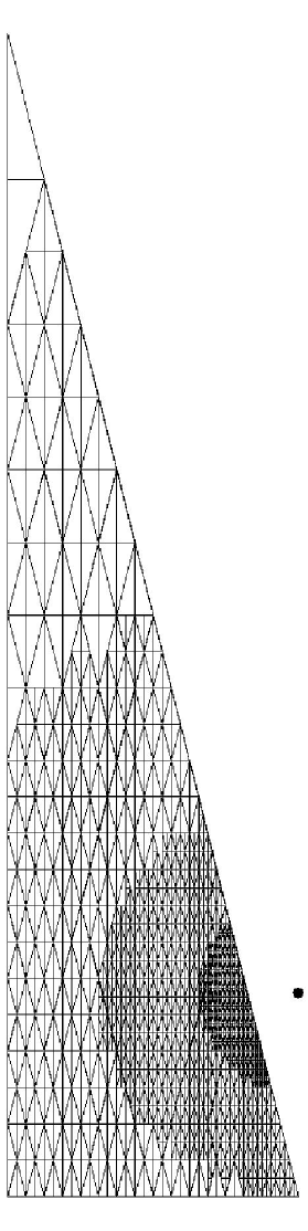
Figure 1: The result of the iterative division of the right-angled triangle with the vertices A=(1,0,0), B=(0,4,0), C=(0,0,0) for the computation of the potential at the point T=(1,0.7,0), denoted by the heavy dot.

The integral $I_{ij}$ of the right-angled triangle up to the quadrupole contribution at the point $\vec{x_{i}}$ is given by the expression

$$I_{ij}=k\left[\frac{1}{\mid\vec{x_{i}}-\vec{x_{j}}\mid}+\frac{1}{6}Q_{mn}\frac{(\vec{x_{i}}-\vec{x_{j}})_{m}(\vec{x_{i}}-\vec{x_{j}})_{n}}{\mid\vec{x_{i}}-\vec{x_{j}}\mid^{5}}\right]\,.$$ (10)

The expression given above is applicable for surface elements $i$ and $j$ sufficiently far apart. However, if these elements are close, this approximation may not suffice for some predefined accuracy in the calculation of the potential. The criterion for the applicability of the expression (10) is that the ratio of the distance $\mid\vec{x_{i}}-\vec{x_{j}}\mid$ to the typical size of the right-angled triangle is larger than some number. The measure of the size of the right-angled triangle is taken to be the larger of its catheti. According to our numerical analysis, when the value of the ratio of $\mid\vec{x_{i}}-\vec{x_{j}}\mid$ and the larger cathetus (let us denote it by $\eta$) is $\geq 5.5$, the quadrupole corrected monopole term (10) gives the approximation of the result obtained by the direct numerical integration with an accuracy of $10^{-4}$. Furthermore, when the ratio $\eta$ is $\geq 26$, the monopole term alone is sufficient to provide the approximation with the same accuracy. These findings are valid for all right-angled triangle shapes, i.e. for all ratios of the larger and smaller catheti. Therefore, if the ratio $\eta$ is $\geq 26$, the monopole term is used and if the afore-mentioned ratio is $\geq 5.5$, the monopole plus quadrupole terms are used. If, however, we have $\eta<5.5$, the right-angled triangle is divided into four similar right-angled triangles obtained by the bisections of the sides of the original right-angled triangle. It is important to note that the respective $\eta$ ratios of the four newly formed right-angled triangles are generally larger than those of the original triangle. The procedure is then repeated for each of the four right-angled triangles and subsequently iterated until all obtained right-angled triangles satisfy the condition $\eta\geq 5.5$. The result of one such iterative division for an elongated right-angled triangle and a nearby point is shown in Fig. 1. Summation of contributions of all triangles yields the final result. At this place it is important to stress that the subdivision of the right-angled triangle depicted in Fig. 1 is not a rafinement of the discretization of the surface, but only an auxiliary tool during the calculation of the potential. The combination of the multipole expansion up to the quadrupole and the iterative division of the triangle surface provides a fast, reliable and robust method for the calculation of $I_{ij}$ quantities.

During the entire execution of the RH method only the potentials at all POCs are stored. The quantities $I_{ij}$ are calculated over again at each instance when they are needed, i.e. they are not recorded at any instant during the execution of the algorithm. If the algorithm of the method should include storing of the quantities $I_{ij}$, memory requirements would grow quadratically with the number of surface elements $N$. In this case, an advantage would be that these quantities would have to be calculated only once. However, we do not adopt this approach. Since only potentials are recorded in the RH method, memory requirements grow linearly with $N$. This feature is clearly a large advantage. The disadvantage lies in the necessity of a new calculation of the quantities $I_{ij}$ whenever they are needed. However, owing to the essential characteristics of the RH method, this disadvantage is not so severe. Namely, the algorithm of the RH method can be divided into two stages. In the first initializational stage, the values of the potential are calculated at all POCs from some initial charge distribution. In this stage the number of required calculations of the quantities $I_{ij}$ grows as $N^{2}$ (it is important to note that the times necessary for all these calculations are not the same). In the second stage, the iterative non-local charge transfers are made. A very important characteristic of the RH method emerges in this stage. The potentials at all POCs after any iteration (charge transfer) need not be completely calculated, but only updated. Namely, it is only necessary to add changes due to the charge transferred between the two chosen POCs. In this update the number of required calculations of $I_{ij}$ scales as $N$. In this way, the potential is largely reused from one iteration to the other. This feature of the potential updating is at the core of the many powerful characteristics of the RH method. Recalculation of $I_{ij}$ at every step fully justifies great attention that was paid to the choice of the optimal method for the calculation of these quantities, which was elaborated in the preceding paragraphs. The choice of the optimal calculational method for $I_{ij}$, together with the updating feature described above, makes the execution times of the RH method acceptable.

The RH method has also attractive properties with respect to parallelization. In the parallelized version of the RH method, each of the processors would be assigned a subset of surface elements. The advantages of parallelization can be seen, e.g. in the update of the potential. Once in some iteration the charge transfer is performed, each of the processors simultaneously calculates the update of the potential in its realm. The possibility of efficient parallelization also significantly improves the execution time of the RH method.

Another rafinement of the method is available if we consider the dynamical approach to the division of the studied surface into triangles. In the present paper, the initial division depends only on the surface geometry, while it is completely insensitive to physical quantities. In such a setting, it is possible that an approximation of some conducting surface even with a large number of triangles may in some areas where physical quantities have large gradients be inadequate and locally provide results of lower quality. Clearly, the solution of this problem is in dividing the existing triangles into smaller ones in the areas where the refinement is needed. Within our method, it is especially easy to accommodate this form of refinement of the approximation of the studied surface with a set of right-angled triangles. There are two principal reasons for this. The solution satisfying the condition of equipotentiality for the cruder set of triangles can be used as a starting distribution for the iteration with the refined set of triangles. This further accelerates the computation. Furthermore, it is straightforward to specify criteria which determine which triangles should be further divided. Thus the iteration procedure naturally leads to the determination of areas where the refinement is required. One criterion might be that the percentage $\alpha$ of all triangles with the largest charges are further divided. Another criterion might be to consider the average or overall difference of the potential at the vertices of the triangle and its POC. For example, one might consider the quantity $G_{i}=(U(\vec{x_{i}})-U(\vec{x_{i}}^{A}))^{2}+(U(\vec{x_{i}})-U(\vec{x_{i}}^{B}))^{2}+(U(\vec{x_{i}})-U(\vec{x_{i}}^{C}))^{2}$, where $\vec{x_{i}}$ denotes the POC of the triangle $i$, while $\vec{x_{i}}^{A,B,C}$ stand for its vertices. In this case, further division would be performed on those triangles for which $G_{i}^{1/2}/U(\vec{x_{i}})\geq\beta$, where $\beta$ is a predefined factor. The entire computational scheme would then include iterations of a composite procedure: for a given set of triangles, the equipotentiality at their POC would be achieved and then, using one of the criteria specified above, the set of triangles would be refined by the division of some of them. The application of this composite iterative procedure yields a powerful computational method for interesting classes of electrostatic (and other) problems.

The adaptive subdivision, as described in the preceding paragraph, refines only the set of triangles obtained in the initial discretization of the surface. The vertices of the new triangles lie in the planes of the old triangle, not on the original surface , which is in general case curved. The procedure that discretizes the surface just produces the set of triangles, and the RH method uses these triangles during the entire execution and possible adaptive subdivision. The set of triangles is an input for the RH method. The full adaptive approach would have to include the refinement of the surface discretization and not only the subdivision of the initial discretization of the surface. In such an approach it becomes necessary to integrate the discretization procedure with the RH method. This approach has not been pursued in this paper that serves as an introduction to the RH method. For the high precision technical applications, such as e.g. investigation of “hot spots”, this approach needs to be adopted.

4 Examples

The main goal of this section is to display solutions obtained using the RH method. For each characteristic of the method we specify examples demonstrating its advantages. In some of the examples given below, the units of dimensional quantities are left unspecified since the results are valid for arbitrary units.

4.1 Comparison with analytic results

In this subsection we discuss solutions of two problems obtained by our computational method and compare the numerical results with the analytical solutions. To bring up several points we choose two significantly different problems:

• a metal grounded sphere of radius $R$, centered at the origin and a point charge $q$ at a distance $y$ from the centre of the sphere ($y>R$)

• two infinite parallel metal cylinders, one completely inside the other as shown in Fig. 2. The outer cylinder is charged with charge +Q and the inner with -Q i.e. they form a capacitor.

The first problem is easily accessible by the RH numerical method due to the finite size of the objects involved in the calculation (the sphere and the point charge). This problem is analytically solved in detail in [1] using the method of images. The induced charge on the sphere has value $q_{ind}=-qR/y$. Our solution for the parameters $y=3$, $R=2$, $q=10$ and the sphere represented by 139240 triangles yields $q_{ind}=-6.6664$ while the exact value is $-20/3=-6.666666$ which is 0.004$\%$ difference.

The second problem of capacitance of two infinite cylinders can not be done in numerical calculation without approximation of the infinite cylinders by the finite ones. Using the finite instead of the infinite cylinders will introduce the charge distribution at the ends of the cylinders different from the one obtained in exact analytical solution for infinite cylinders. Nevertheless, one can efficiently eliminate the contribution of these boundary effects in the final solution for the capacitance per unit length. Generally, when we calculate capacitance of some system, we put charges of equal size and different sign (namely $+Q$ and $-Q$) on two objects representing the “plates” of the capacitor and then solve for the equipotentiality of each of these isolated charged objects. By that we obtain the potential of each plate and the potential difference U between the capacitor plates. The capacity of such a system is then given by definition as $C=Q/U$. In this case we know that the calculated system is different from the infinite system and that the main difference is in boundary effects that are present in the numerical solution. Therefore we perform two calculations with different lengths of cylinders. The boundary effects contribution to capacitance of the system can be canceled and we can obtain a very accurate value of $C/L$ for the infinite cylinders in the following way: if the capacitance in the calculation in which the length of the cylinders is $L_{1}$ is $C_{1}$ and the capacitance of the cylinders of length $L_{2}$ is $C_{2}$ then the capacitance of the infinite capacitor per unit length L would be

$$\frac{C}{L}=\frac{C_{2}-C_{1}}{L_{2}-L_{1}}.$$ (11)

One can solve this problem analytically by the method of images replacing two cylinders with two homogeneously charged wires at positions A and B as shown in Fig. 2 and require for a constant potential at each cylindrical surface. The obtained solution gives capacitance per unit length

$$\left(\frac{C}{L}\right)^{-1}=2\ln\left(\frac{R_{1}^{2}+R_{2}^{2}-d^{2}+\sqrt{R_{1}^{4}+R_{2}^{4}+d^{4}-2d^{2}R_{1}^{2}-2d^{2}R_{2}^{2}-2R_{1}^{2}R_{2}^{2}}}{2R_{1}R_{2}}\right)$$ (12)

The two calculations were performed with the following parameters: i) for $d=0.25$, $R_{1}=1.0$, $R_{2}=0.25$, $L_{1}=15.6$ and both cylinders represented by N=75000 triangles, the obtained capacitance per unit length is $C_{1}/L_{1}$=0.391198. ii) for $d=0.25$, $R_{1}=1.0$, $R_{2}=0.25$, $L_{1}=19.6$ and both cylinders represented by N=75000 triangles, the obtained capacitance per unit length is $C_{2}/L_{2}$=0.394214.

When we calculate $C/L$ as given in equation (11), we obtain $C/L=0.379433$ which is only $0.06\%$ different from the analytical value.

We shall exploit this example further to demonstrate how the RH method finds the distribution of surface charge in such a system which possesses the mirror plane symmetry (it can also have axial symmetry in case of concentric cylinders i.e. when $d=0$). In the analytical solution one can find the electric potential and the electric field everywhere in the space and particularly at the surface of the cylinders. From the value of the electric field at the cylinder surfaces one can find the surface charge on them. We compare the surface charge of the outer cylinder found by the RH method with the values from the analytical solution. Due to the boundary effects, we choose for comparison one slice from the middle of the cylinder as shown in Fig. 2. In Fig. 3 is given the comparison between the numerical and the analytical solution for the surface charge. The agreement is very good, considering that the analytical solution is obtained for infinite cylinders. To show how the RH solution respects the symmetry of the system, we calculate the electric potential and the electric field in the plane perpendicular to the axes of cylinders and passing through the middle of their length. The symmetry of the RH solution perfectly respects the symmetry of the problem even though in the RH method information on symmetry on the problem is not imposed in any way and enters the calculation process only through the positions of input triangles.

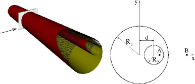
Figure 2: The geometrical configuration of the cylinders forming the capacitor. The arrow in the left picture shows the slice for which the potential and the electric field are calculated and shown in Fig. 4

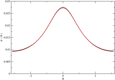
Figure 3: The angular dependence of the surface charge density of the outer cylinder. The very good agreement of the numerical and the analytical curve is evident.

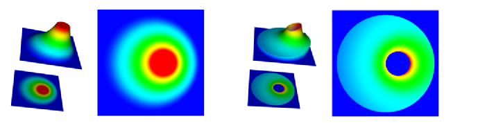
Figure 4: Once the distribution of the surface charge is found by the RH method, one can calculate the electric potential (three figures on the left) and the electric field (three figures on the right) in the whole space which is very important in the study of discharge, “hot spots”, etc. In the set of pictures describing the electric field, the absolute value of the electric field vector is shown. The calculations were done for the slice shown in Fig. 2

4.2 Potential problems in complex configurations and geometries

In this subsection we present solutions of several potential problems with complex configurations and geometries. These examples are designed to illustrate that the numerical method introduced in this paper can quite easily handle even very demanding geometries and configurations, i.e. shapes and relative positions of the conducting surfaces.

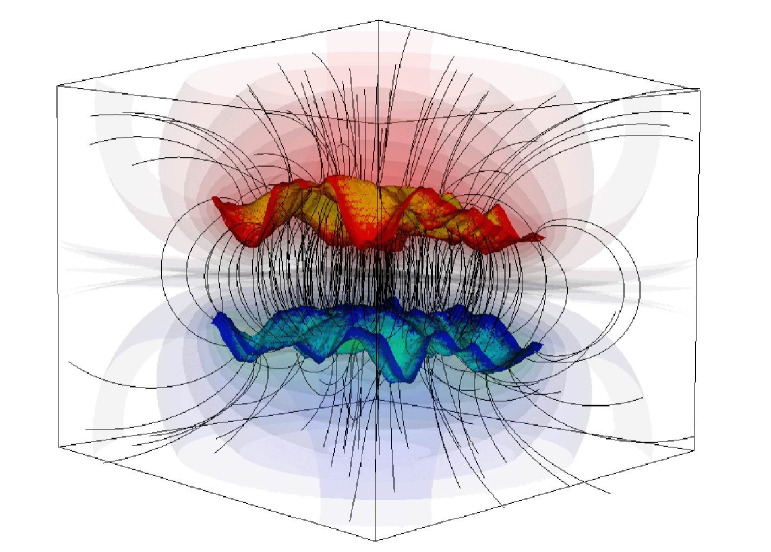
Figure 5: The surface charge density, the equipotential surfaces and the lines of force for the system of two insulated randomly generated surfaces with charges $+Q$ and $-Q$. The random surfaces were generated using the Perlin noise algorithm contained in the VTK program package [11]. The colours towards red correspond to positive charge densities and the colours towards blue correspond to negative charge densities.

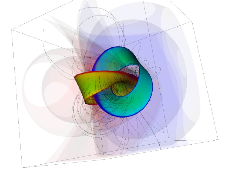
Figure 6: The surface charge density, the equipotential surfaces and the lines of force for the system of two Möbius stripes with charges $+Q$ and $-Q$. The colours towards red denote to positive charge densities and the colours towards blue denote negative charge densities.

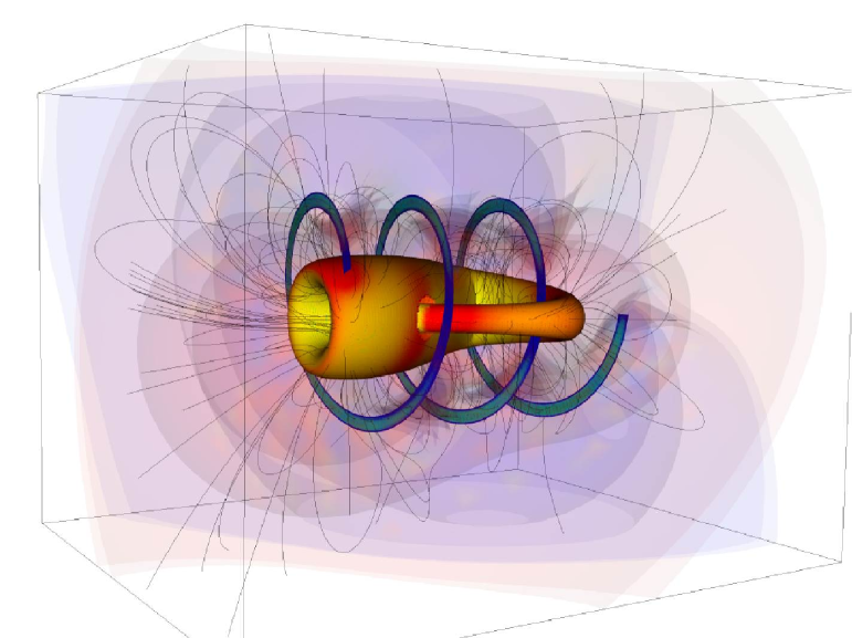
Figure 7: The surface charge density, the equipotential surfaces and the lines of force for the system of a segment of a spiral and a Klein bottle with charges $+Q$ and $-Q$. The colours towards red represent positive charge densities while the colours towards blue represent negative charge densities.

We study three different systems of which each consists of two insulated conducting surfaces. One of the surfaces carries the charge $+Q$ while the other carries the charge $-Q$. In this way, each of three studied systems represents a capacitor. In all three cases, shown in Figs 5, 6 and 7, the colours towards red stand for positive charge densities while the colours towards blue represent negative charge densities.

The first system consists of two randomly generated surfaces. The solution in terms of the surface charge densities, equipotential surfaces and the lines of force is depicted in Fig. 5. The RH method handles without difficulty randomly generated surfaces which confirms its suitability for the treatment of geometries with high degree of variability or irregularity. It is easy to extrapolate how the elaboration of this example might be used in realistic systems with irregular surfaces.

The second system consists of two interlocked Möbius stripes, as displayed in Fig. 6. By itself it is a purely academic example, which, however in our case demonstrates the effectiveness of the RH method in more complex topologies. Namely, Möbius stripe has no inner and outer surface, as opposed to other surfaces considered so far. Figure 6 shows the equilibrium surface charge densities, the equipotential surfaces and the lines of force.

The third system includes a segment of a spiral intertwined with a “Klein bottle”. The purpose of this example is to show how far the geometric complexity of the system can be pushed using the RH method. The equilibrium situation for this system comprising the surface charge densities, equipotential surfaces and the lines of force is given in Fig. 7.

The examples given in this subsection demonstrate how RH method handles even geometrically very complicated situations. The results presented so far show that the RH method is a robust method which can be used in treatment of very different geometries.

5 Technical characteristics of the method

In the preceding section we demonstrated the applicability of our method to a broad range of different configurations (arrangements of objects in space) and geometries (shapes of individual objects), charge distributions and potential boundary conditions, as well as its reliability by comparisons with analytic solutions for selected problems. In this section we focus on technical characteristics of the method.

Figure 8: The computational complexity of the RH method. a) The dependence of the execution time of the first stage $t_{1}$ on the number of triangles $N$ for the system of the conducting sphere at a fixed potential and the point charge. b) The execution time of the second stage $t_{2}$ as a function of $N$ for the same system as in a). c) The dependence of $t_{1}$ on $N$ for the system of a point charge and a plane at a fixed potential. d) The dependence of $t_{2}$ on $N$ for the same system as in c).

One of the most prominent characteristics of any algorithm is its complexity. It specifies how the execution time of the algorithm changes depending on the number of elements that the algorithm deals with. The complexity of our method determines how the time required to achieve the equipotentiality in the system scales with the number of surface elements $N$ for a specified geometry. To make a more thorough analysis of the computational complexity of the RH method, we chose to measure the dependence of the time of the execution of two stages in the algorithm of the RH method on the number of surface elements $N$. The first stage is the calculation of the initial potential at the surfaces of the considered system, while the second stage comprises successive iterations of the non-local transfer of the charge until equipotentiality is achieved. To account for possible dependence of the complexity on the geometry, we studied several geometries and configurations. For each total number of surface elements $N$, the initial division of the surfaces was used throughout the calculation, i.e. no iterative subdivisions of the surface elements described in section 3 were used. Both the execution time of the first stage, $t_{1}$ and the execution time of the second stage, $t_{2}$, are well described by the power laws, i.e. $t_{i}\sim N^{\alpha_{i}}$, $i=1,2$. The first system in which the investigation of the complexity of the RH method was performed is the system of a point charge near a conducting sphere at a fixed potential. In this system, the exponents are $\alpha_{1}=1.62$ and $\alpha_{2}=1.58$. For the system of the conducting plane kept at the exterior potential and a point charge and a similar system of the insulated plane and a point charge, we obtain very similar results. The exponents of the first stage are $\alpha_{1}=1.70$ and the exponents of the second stage amount to $\alpha_{2}=1.64$ for both systems. The log-log plots illustrating complexity for the specified systems are presented in Fig. 8. The exponents $\alpha_{i}$ of the two stages are generally different, where $\alpha_{1}$ is slightly larger than $\alpha_{2}$ for all studied systems. The results obtained show that the complexity is geometry dependent. The complexity difference of the two studied geometries is not large, but the general dependence of the complexity on geometry is an open question. Very similar results for the systems containing conducting planes indicate that there is no significant dependence of complexity on potential configuration. These results imply that RH method has no intrinsic complexity, but it is system dependent. However, a very important characteristic of the RH method emerges from the results of the studied systems. In all studied cases, the largest of the two exponents (which determines the complexity of the entire RH method) is considerably less than 2 for $N$ of the order of $100$ to the order of $10^{5}$. This feature, boosted by the easy parallelization and adaptive subdivision, makes the RH method competitive for large-scale problems involving a large number of surface elements.

A significant advantage of the method introduced in this paper is connected with memory requirements for calculations with $N$ surface elements. Namely, the required memory scales linearly with $N$, which is a tremendous reduction of the required memory capacitance compared with, e.g. the existing BEM, where the required memory scales as $N^{2}$. Even with a single processor, using our method it was possible to easily perform calculations with $N=2\cdot 10^{5}$ surface elements .

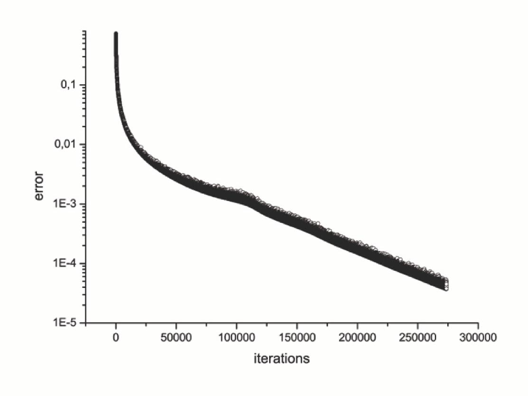
Figure 9: The speed of convergence for the system of the point charge close to the sphere kept at a fixed potential. The exponential character of the error reduction with the number of iterations is evident. There is no effect of the Critical Slowing Down and the error reduction efficiency is the same for any level of the error.

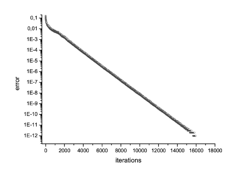
Figure 10: The speed of convergence for the system of the point charge located close to the insulated conducting sphere. The error decreases exponentially with the number of iterations for a broad range of error orders of magnitude. There is no effect of the Critical Slowing Down.

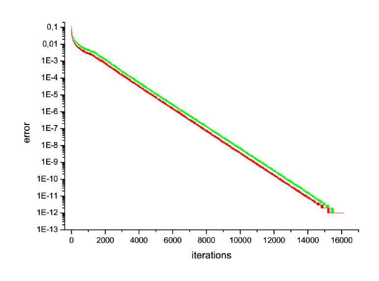
Figure 11: The speed of convergence for the system of a point charge and two insulated conducting spheres (upper curve) compared with the speed of convergence of the system discussed in Fig. 10 (lower curve). In both cases, the error decreases exponentially with the number of iterations. The addition of one more separate conducting surface does not deteriorate the speed of convergence.

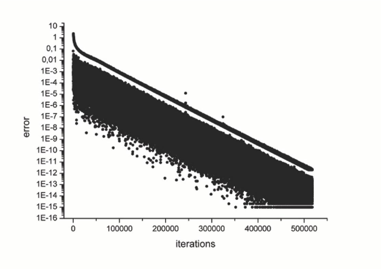
Figure 12: The speed of convergence for the system of a two randomly generated surfaces with charges of the equal amount and opposite sign. The error decreases at worst exponentially with the number of iterations without the CSD effect.

A further important advantage is related to the speed of convergence of the method. The speed of convergence was studied in three different systems which all exhibit similar convergence properties. The first system consists of a charge close to a sphere kept at a fixed potential. The behaviour of the error of the potential (defined as $(U_{\mathrm{maxdiff}}-U_{\mathrm{ext}})/U_{\mathrm{ext}}$ at a given iteration, where $U_{\mathrm{ext}}$ is the external potential and $U_{\mathrm{maxdiff}}$ is the potential differing the most from $U_{\mathrm{ext}}$) as a function of the number of iterations performed, which is quite accurately equivalent to the execution time, is given as a log-lin plot in Fig. 9. From the figure it is clear that the error decreases exponentially with the number of iterations. An analogous graph for the system of the point charge close to an insulated conducting sphere is depicted in Fig. 10. The exponential dependence of the decrease of error on the number of iterations is evident. Finally, we consider a system consisting of a point charge and two insulated conducting spheres. In this system each sphere ends up in a state with its own potential and charge redistribution is performed separately within each sphere. The error of the potential decays with the number of iterations in this case as well. Since we have two separate bodies on which the potentials have to be equalized separately, it is reasonable to ask if the method converges more slowly than for the system where the potential has to be equalized on a single surface only. To answer this question, in Fig. 11 we present the dependence of the error of the potential on the number of iterations for the system with two spheres (the upper curve) and for the system with one sphere (the lower curve), which has already been presented in Fig. 10. This graph very clearly shows that the speed of convergence is the same for both systems. To complete the analysis of the speed of convergence, we studied the system consisting of two insulated conducting randomly generated surfaces carrying charges $+Q$ and $-Q$. The results obtained are very similar to the preceding cases as shown in Fig. 12. Namely, for both surfaces the convergence is at worst exponential. The larger dissipation of points in the graph reflects the random nature of the studied geometry. The facts stated above indicate that our method handles systems of a different degree of geometric and configurational complexity with the same convergence speed, which is a very welcome property. It is important to state one additional convergence property common to Figs 9, 10, 11 and 12. The dependence of the error on the number of iterations is a straight line in the log-lin plot for a broad range of iteration numbers. In other words, no matter how small the error is, it is reduced by more or less the same percentage at subsequent iteration. The method has the same efficiency of error reduction for all error sizes. Equivalently, the RH method equally well reduces the error of the potential at the beginning of the calculation and at its end. Therefore, there is no effect of the Critical Slowing Down (CSD) present in some calculational methods [13, 14], where the use of the local information for the solution update leads to significant reduction in the convergence speed with the number of iterations. This deficiency has been overcome using the multigrid techniques [16] which, however, require additional adjustment procedures. From the principles of the RH method it is clear that the update of the potential is based on the global information on the studied system. The absence of CSD could be explained by completely non-local charge transfers that always affect the two worst points in the system making them the best points according to the criteria of equipotentiality. One of the reasons of the very fast convergence is a natural adaptation of quantity of charge transfer being done at certain potential difference, i.e. at the reached precision. The RH method handles the system equally efficiently at all levels of error. In this sense, the system at a large potential difference of the order of 100 V (which represents a solution far from convergence) represents exactly the same problem for the method as the same system when it has reached differences of $10^{-20}$ V (already well converged solution) and is being equally efficiently treated by the method. The absence of the CSD, together with the $N$ scaling of the required memory, makes our method very suitable for large-scale high precision calculations.

Finally, we would like to address the technical features of the adaptive subdivision procedure described in section 3. As already described, this procedure achieves equipotentiality with the coarser division of the surface and uses the charge distribution obtained as an initial distribution for the calculations with the finer surface division in the next step. The open question at each step of this procedure is what proportion of triangles will be subdivided and according to which criteria. Some of these criteria were proposed in section 3. We call the sequence of proportions and criteria for each step subdivision strategy. With the subdivision strategy of dividing each right-angled triangle to four similar ones at each subdivision step, we achieved the reduction of the execution time around 25 % for the system of a point charge near a grounded plane. Although the RH method has excellent properties even without adaptive subdivision, the choice of the subdivision strategy is a matter of the further optimization of the entire method.

6 Applications beyond electrostatic problems

The applicability of a numerical method to some physical problems depends on the mathematical formulation of the problem. Many diverse physical problems have an identical (or analogous) mathematical formulation and, therefore, can be treated with the same numerical method. The RH method can be transferred from the class of electrostatic problems to any physical problem with the same mathematical formulation. An obvious application of the RH method beyond electrostatics is thermostatics.

One possibility of extending the field of applicability of the RH method is its transfer to the problems with identical mathematical formulation. However, except transferring the method in its original form, it is possible to modify the RH method maintaining its basic principle of achieving equipotentiality. In the modified RH method, the quantities such as the potential and the charge distribution have to be understood more generally. Let us consider a problem in which it is necessary to find a spatial configuration of the system in its physical state. The role of the potential can be played by a quantity, let us call it the generalized potential, which is spatially constant when the system is in the physical state. The role of the charge distribution is then played by any source, spatial distribution of which has to be determined in order to equipotentialize the generalized potential. These modifications of the RH method allow its application in a very broad range of physical problems. In the following paragraph are given several illustrations of possible applications.

The (modified) RH method can be applied to semiclassical and quantum problems as well. Each new application, apart from the modifications described above, requires some technical adaptations. An example of the application of the RH method in semiclassical problems is the treatment of the Thomas-Fermi approach. In this case, the generalized potential becomes the energy of the system and the source is the density of the particles. The generalized potential depends non-linearly on the density owing to the approximation of the kinetic term. The modified RH method handles this non-linear system equally well as the linear ones. Another example of application is solving one-particle Schrödinger equation in an arbitrary potential. This is an eigenvalue problem which requires additional adaptations of the original RH method. In the definition of the generalized potential appear the terms with derivatives. In the discretized version of the problem, these terms introduce non-locality into the problem. The ground state of the system can be obtained in a straightforward fashion [15]. The problem of excited states and degeneracy is under current study [15]. Finally, there are indications that the modified RH method might be very useful within the DFT approach [16, 17, 18]. Recently, real space DFT methods have emerged [16]. An implementation of real-space DFT based on the RH method is a promising approach for the treatment of electronic structure problems.

7 Conclusions

In this paper we have presented a robust calculational method, which we have named the Robin Hood (RH) method, for solving a large class of problems in electrostatics. The physical basis of the RH method is the very intuitive concept of non-local transfer of the electric charge on the conducting surfaces with the aim of achieving equipotentiality of all conductors. The non-locality of the charge transfer and the long range of the electrostatic interaction make possible the global (i.e. at the level of all conducting surfaces) improvement towards the equipotentiality with each charge transfer. The method is characterized by many technical advantages which promote it into an attractive tool for treating complex problems in electrostatics. The memory requirements grow linearly with the number of surface elements $N$. The complexity of the method itself scales as $N^{\alpha}$ with $\alpha<2$ and is (somewhat) geometry dependent. The speed of convergence is exponential and the Critical Slowing Down is not present, which eliminates the necessity for procedures like multigrid techniques. Our method does not use multigrids [5, 16]. The results of the method are “recyclable” in the sense that the charge distributions which satisfy the condition of equipotentiality at coarse surface divisions can be efficiently used as initial charge distributions for the calculations with finer surface divisions. The adaptive subdivisions of selected surface elements can be easily incorporated into the RH method, which can provide additional increase in the computational efficiency of the method.

Despite many appealing sides of the RH method demonstrated in this paper, there are other issues to be investigated and possibly improved. Although the method is already in many respects optimized, the question of performing charge transfers among more than two points at each conducting surface, in linear problems such as electrostatics, remains. It is not excluded that for some $N_{\mathrm{p}oints}\geq 3$ the RH method delivers even better results, although a conceptually more complex approach. The strategy of the adaptive subdivisions of selected surface elements is another aspect where careful optimization could lead to further improvements. A more detailed study of the dependence of complexity on geometry might shed some light on geometries in which the method would provide an even better performance than for the systems studied in this paper. These matters, along with other technical aspects, clearly constitute important questions worthy of further pursuit.

Besides rather academic examples shown in this paper, the RH method is suitable for the electrostatic calculations of high precision in many practically very important examples such as the design of high energy particle detectors, instruments for medical applications, circuit board design and many others.

Although the RH method is applicable to large classes of problems in electrostatics, it is worth investigating if the method could be modified to encompass some other systems, such as those for which the explicit Green function is not available. The RH method can be easily transferred into the related fields of classical physics and engineering where the mathematical background is equivalent. Furthermore, this method provides a new way of handling quantum phenomena, the one-particle Schrödinger equation and DFT being some of them. Although the strength of the (modified) RH method in quantum problems is still to be properly gauged, it is definitely a new alternative for unraveling the properties of important physical systems.

Acknowledgments. The authors would like to thank dr. Radovan Brako and Prof. Dragan Poljak for useful comments on the manuscript. We acknowledge the use of VTK and Mathematica program packages. This work was supported by the Ministry of Science and Technology of the Republic of Croatia under the contract numbers 0098001 and 0098002.

References

- [1] J.D. Jackson, Classical Electrodynamics, 2nd edition, (John Wiley & Sons, New York, 1975).
- [2] L.D. Landau and E.M. Lifshitz, Electrodynamics of continuous media (Pergamon Press, Oxford, 1993).
- [3] R.P. Feynman, R.B. Leighton and M. Sands, The Feynman Lectures on Physics (Addison Wesley Longman, Reading, Mass., 1970).
- [4] E.M. Purcell, Electricity and Magnetism, in Croatian (Tehnička knjiga, Zagreb, 1988).
- [5] T.L. Beck, Multiscale Tecniques for Electrosatic and Eigenvalue Problems in Real Space, in G. Hummer and L.R. Pratt, eds., Simulation and Theory of Electrostatic Interactions in Solution (AIP Press, New York, 1999).
- [6] D.J. Willis, J.K. White and J. Peraire, A pFFT Accelerated Linear Strength BEM Potential Solver, presented at MSM ’04 7th Int. Conf. on Modeling & Simulation of Microsystems, March 7-11, 2004, Boston MA.
- [7] S-W. Chyuan, Y-S. Liao and J-T. Chen, An Efficient Method for Solving Electrostatic Problems, Computing in Science and Engineering, 5 (2003) 52-58.
- [8] Z. Liu, J.G. Korvink and M. Reed, Solving Singularities in Electrostatics with High-order FEM, IEEE 2003 (Toronto, Canada, 2003).
- [9] http://www.boundary-element-method.com/
- [10] D.Poljak, A. Peratta and C. Brebbia, Eng. Anal. Bound. Elem. 28 (2004) 763; D. Poljak, Eng. Anal. Bound. Elem. 27 (2003) 283.
- [11] http://www.vtk.org
- [12] http://www.wolfram.com
- [13] T. Torsti, M. Heiskanen, M.J. Puska et al., MIKA: Multigrid-based program package for electronic structure calculations, Int. J. Quantum Chem. 91 (2003) 171-176.
- [14] M. Heiskanen, T. Torsti, M.J. Puska and R.M. Nieminen, Multigrid method for electronic structure calculations, Phys. Rev. B 63 (2001) 245106.
- [15] P. Lazić, H. Štefančić and H. Abraham, work in progress.
- [16] T.L. Beck, Real-space mesh techniques in density functional theory, Rev. Mod. Phys. 72 (2000) 1041-1080.
- [17] http://www.fysik.dtu.dk/campos/Dacapo/
- [18] W. Kohn and L.J. Sham, Self-Consistent Equations Including Exchange and Correlation Effects, Phys. Rev. 140 (1965) 1133-1138.