A possibility to measure elastic photon–photon scattering in vacuum

Abstract

Photon–photon scattering in vacuum due to the interaction with virtual electron-positron pairs is a consequence of quantum electrodynamics. A way for detecting this phenomenon has been devised based on interacting modes generated in microwave waveguides or cavities [G. Brodin, M. Marklund and L. Stenflo, Phys. Rev. Lett. 87 171801 (2001)]. Here we materialize these ideas, suggest a concrete cavity geometry, make quantitative estimates and propose experimental details. It is found that detection of photon-photon scattering can be within the reach of present day technology.

I Introduction

Classically, photon–photon scattering does not take place in vacuum. However, according to quantum electrodynamics (QED), such a process may occur owing to the interaction with virtual electron–positron pairs. An effective field theory containing only the electromagnetic fields can be formulated in terms of the Heisenberg–Euler Lagrangian Heisenberg-Euler ; Schwinger , which is valid for field strengths below the QED critical field $10^{18}\,\mathrm{V\,m^{-1}}$ and for wavelengths shorter than the Compton wavelength $10^{-12}\,\mathrm{m}$ general ; general2 ; general3 . Several suggestions to detect photon-photon scattering in laboratories have been made Older ; Older2 ; Older3 , and the recent increase in available laser intensities has stimulated various schemes Recent ; Recent2 ; Recent3 ; Recent4 ; Recent5 ; Recent6 . In Ref. Brodin-Marklund-Stenflo we suggested an alternative method, using the significantly weaker (but still strong) fields that can be confined in a microwave cavity. The main advantage of adopting a cavity is that we can achieve a resonant interaction between the eigenmodes in a large volume, leading to an excited signal at a new eigenfrequency.

In the present paper we materialize the proposal made in Ref. Brodin-Marklund-Stenflo in several ways. Various concrete geometries fulfilling all resonance and frequency matching conditions in a cavity are devised, and the coupling between the pump modes and the excited mode is evaluated for a rectangular prism and a cylindrical geometry. The amplitude of the excited mode is then determined in terms of the quality factor of the cavity and the field strengths of the pump modes. Comparing with the performance reached in existing superconducting niobium cavities, it turns out that the cavity key parameters, namely the quality factor and the allowed field strength (before field emission and/or superconductivity break down) can reach values which allow for several photons in the excited mode. To be able to detect the very weak excited signal in the presence of the pump waves, we propose a ”cavity filtering geometry”. Finite element calculations are made in order to demonstrate a geometry that fulfills the relevant resonance and frequency matching conditions. The estimated signal in the filtered region corresponds to roughly 30 microwave photons/$\mathrm{m}^{3}$. The results of Refs. Q-factor1 and NOGUES99 , where effects of single microwave photons confined in cavities are measured using sensitive techniques involving transitions of Rydberg atoms, suggest that detection of the estimated signal is possible. Hence we suggest that elastic photon-photon scattering can be observed with present day technology.

II Basic equations and principles of calculation

Photon-photon scattering due to the interaction with virtual electron positron pairs can be described by the Heisenberg–Euler Lagrangian Heisenberg-Euler

$$L=\varepsilon_{0}F+\kappa\varepsilon_{0}^{2}\left[4F^{2}+7G^{2}\right]$$ (1)

where $F=(E^{2}-c^{2}B^{2})/2$ and $G=c\mathbf{E}\cdot\mathbf{B}$. Here $\kappa\equiv 2\alpha^{2}\hbar^{3}/45m_{e}^{4}c^{5}\approx 1.63\times 10^{-30}\,\mathrm{m}\mathrm{s}^{2}/\mathrm{kg}$, $\alpha$ is the fine-structure constant, $\hbar$ Planck’s constant, $m_{e}$ the electron mass, and $c$ the velocity of light in vacuum. The last terms in (1) represent the effects of vacuum polarization and magnetization. The QED corrected Maxwell’s vacuum equations can then be written in their classical form using $\mathbf{D}=\varepsilon_{0}\mathbf{E}+\mathbf{P}\$and $\mathbf{H}=\mathbf{B/}\mu_{0}-\mathbf{M}$  where $\mathbf{P}$ and $\mathbf{M}$ are of third order in the field amplitudes $\mathbf{E}$ and $\mathbf{B}$, and $\mu_{0}=1/c^{2}\varepsilon_{0}$. Expressions for $\mathbf{P}$ and $\mathbf{M}$ can be found in, for example, Refs. general ; general2 ; general3 ; Older ; Older2 ; Older3 ; Recent ; Recent2 ; Recent3 ; Recent4 ; Recent5 ; Brodin-Marklund-Stenflo .

There are several reasons for considering wave interactions in cavities:

1. We can benefit from coherent resonant interactions. In contrast, the nonlinear coupling vanishes for parallell plane waves in an unbounded medium. However, we note that the presence of an inhomogeneous background magnetic field can also be responsible for a nonzero effect, see Ref. Recent6 .

2. The growth of the new mode will not be saturated by convection out of the interaction region.

3. The techniques for detecting small signals in such cavities are very well developed, see e.g. Refs Q-factor1 ; NOGUES99 .

Calculations of the coupling strength between various eigenmodes can be made including the nonlinear  polarization and magnetization, see e.g. Ref. Brodin-Marklund-Stenflo . However, a more convenient approach, which gives the same result, starts directly with the Lagrangian density (1).

Our general procedure for finding the cavity eigenmode coupling and the saturated amplitude of the excited mode, to be applied in sections III and IV, can be summarized as follows:

1. We determine the linear eigenmodes of the cavity using the standard Maxwell vacuum equations together with the boundary conditions for infinitely conducting walls, and express all field components in terms of the vector potential amplitude.

2. Next we choose resonant eigenmodes fulfilling frequency matching conditions. For two interacting initial pump modes (indices 1 and 2) with distinct frequencies $\omega_{1}$ and $\omega_{2}$, the possible frequency matching choices, corresponding to a cubic nonlinearity, are $\pm(2\omega_{1}\pm\omega_{2})$ and $\pm(\omega_{1}\pm 2\omega_{2})$. For definiteness we concentrate on the choice

$$\omega_{3}=2\omega_{1}-\omega_{2}$$ (2)

in all examples. Since the eigenfrequencies are determined by the geometry, we note that the condition (2) gives a design requirement involving the dimensions of the cavity. In this context it can be noted that there are several reasons for using two pump waves rather than one, that in principle could excite a mode with three times the frequency of the pump mode. Firstly, for two pump modes there are generally better possibilities to vary the parameters in the set-up in order to optimize the output of the excited mode. Secondly, for a cylindrical geometry and a single pump mode, the design requirements following from the frequency matching results in eigenmodes that have a too weak nonlinear coupling. Finally, there is a general tendency to get stronger nonlinear coupling when the pump modes and the excited mode have rather close frequencies.

3. We then perform a variation of the amplitude of the eigenmodes and let $\delta\!\int L\,d^{3}rdt=0$ in order to obtain the mode-coupling equations directly from the Lagrangian density (1). The evolution equation for each eigenmode is obtained by expressing the Lagrangian in terms of the potential and varying the corresponding vector potential amplitude. The lowest order linear terms then vanish, since the dispersion relation of each mode is fulfilled. For the terms that are quadratic in the fields we must thus take into account that the amplitude has a weak time dependence when making the amplitude variation. However, for the QED correction terms in the Lagrangian the time dependence of the amplitudes can be neglected.

4. In the absence of dissipation, the equations now obtained imply steady growth of mode 3, until the energy of that mode is comparable to that of the pump modes. However, when some damping mechanism is present (e.g. due to a finite conductivity of the cavity walls) the amplitude saturates at a level where the mode-coupling growth balances the dissipation of the excited mode. This effect can be easily included by adding a phenomenological damping term in the evolution equation, whose value is estimated by comparing with quality factors currently reached in superconducting niobium cavities.

III Rectangular prism geometry

We start by considering a rectangular prism cavity, with one of its corners in the origin, and the opposite corner with coordinates $(x_{0},y_{0},z_{0})$. In practice we are interested in a shape where $z_{0}\gg x_{0},y_{0}$ but this assumption will not be used in the calculations. We let the large amplitude pump modes have vector potentials of the form

$$\mathbf{A}_{1}=A_{1}\sin\left(\frac{\pi x}{x_{0}}\right)\sin\left(\frac{n_{1}\pi z}{z_{0}}\right)\exp(-\mathrm{i}\omega_{1}t)\widehat{\mathbf{y}}+\mathrm{c.c}$$ (3)

and

$$\mathbf{A}_{2}=A_{2}\sin\left(\frac{\pi y}{y_{0}}\right)\sin\left(\frac{n_{2}\pi z}{z_{0}}\right)\exp(-\mathrm{i}\omega_{2}t)\widehat{\mathbf{x}}+\mathrm{c.c.}$$ (4)

where $\mathrm{c.c.\,}$ denotes complex conjugate, $n_{1,2}=1,2,3...$, and where we have chosen the radiation gauge such that the scalar potential is zero. It is easily checked that the corresponding fields (omitting the c.c.)

$$B_{1z}\!\! = \!\!\frac{\pi}{x_{0}}A_{1}\,\cos\left(\frac{\pi x}{x_{0}}\right)\sin\left(\frac{n_{1}\pi z}{z_{0}}\right)\exp(-\mathrm{i}\omega_{1}t),$$ (5a)

$$B_{1x}\!\! = \!\!-\frac{n_{1}\pi}{z_{0}}A_{1}\sin\left(\frac{\pi x}{x_{0}}\right)\cos\left(\frac{n_{1}\pi z}{z_{0}}\right)\exp(-\mathrm{i}\omega_{1}t),$$ (5b)

$$E_{1y}\!\! = \!\!\mathrm{i}\omega_{1}A_{1}\sin\left(\frac{\pi x}{x_{0}}\right)\sin\left(\frac{n_{1}\pi z}{z_{0}}\right)\exp(-\mathrm{i}\omega_{1}t),$$ (5c)

together with $$\omega_{1}^{2}=n_{1}^{2}\pi^{2}c^{2}/z_{0}^{2}+\pi^{2}c^{2}/x_{0}^{2}$$, and

$$B_{2z}\!\! = \!\!-\frac{\pi}{y_{0}}A_{2}\,\cos\left(\frac{\pi y}{y_{0}}\right)\sin\left(\frac{n_{2}\pi z}{z_{0}}\right)\exp(-\mathrm{i}\omega_{2}t),$$ (6a)

$$B_{2y}\!\! = \!\!\frac{n_{2}\pi}{z_{0}}A_{2}\sin\left(\frac{\pi y}{y_{0}}\right)\cos\left(\frac{n_{2}\pi z}{z_{0}}\right)\exp(-\mathrm{i}\omega_{2}t),$$ (6b)

$$E_{2x}\!\! = \!\!\mathrm{i}\omega_{2}A_{2}\sin\left(\frac{\pi y}{y_{0}}\right)\sin\left(\frac{n_{2}\pi z}{z_{0}}\right)\exp(-\mathrm{i}\omega_{2}t),$$ (6c)

together with $$\omega_{2}^{2}=n_{2}^{2}\pi^{2}c^{2}/z_{0}^{2}+\pi^{2}c^{2}/y_{0}^{2}$$  are proper eigenmodes fulfilling Maxwells equations and the standard boundary conditions. Similarly we assume that the mode to be excited can be described by a vector potential

$$\mathbf{A}_{3}=A_{3}\sin\left(\frac{\pi y}{y_{0}}\right)\sin\left(\frac{n_{3}\pi z}{z_{0}}\right)\exp(-\mathrm{i}\omega_{3}t)\widehat{\mathbf{x}}+\mathrm{c.c.}$$ (7)

where $\omega_{3}^{2}=n_{3}^{2}\pi^{2}c^{2}/z_{0}^{2}+\pi^{2}c^{2}/y_{0}^{2}$, in which case we get fields of the same form as in Eqs. (6a)–(6c).

Next we turn to point three in the scheme of the previous section. As noted above, when performing the variations $\delta A_{3}^{\ast}$, the lowest order terms proportional to $\delta A_{3}^{\ast}A_{3}$ vanish due to the dispersion relation, and we need to include terms due to the time dependence of the amplitude of the type $A_{3}\partial(\delta A_{3}^{\ast})/\partial t$. For the fourth order QED corrections proportional to $\delta A_{3}^{\ast}$, only terms proportional to $A_{1}^{2}A_{2}^{\ast}\delta A_{3}^{\ast}$ survive the time integration, due to the frequency matching (2). After some algebra the corresponding evolution equation for mode 3 reduces to

$$\frac{dA_{3}}{dt}=-\frac{\mathrm{i}\varepsilon_{0}\kappa\omega_{3}^{3}}{8}K_{\mathrm{rec}}A_{1}^{2}A_{2}^{\ast}$$ (8)

where the dimensionless coupling coefficient $K_{\mathrm{rec}}$ is

$$K_{\mathrm{rec}} = \frac{\pi^{2}c^{2}}{\omega_{3}^{4}}\Bigg{\{}(-,-,+)\bigg{[}\frac{8\pi^{2}c^{2}}{x_{0}^{2}y_{0}^{2}}+\left(\frac{4}{x_{0}^{2}}+\frac{7n_{1}^{2}}{z_{0}^{2}}\right)\omega_{2}\omega_{3}\bigg{]}+\frac{n_{2}n_{3}\pi^{2}c^{2}}{z_{0}^{2}}\left(\frac{7n_{1}^{2}}{z_{0}^{2}}-\frac{3}{x_{0}^{2}}\right)$$ (9)

$$+\frac{7\omega_{1}n_{1}}{z_{0}^{2}}\left((-,+,-)\omega_{2}n_{3}(+,-,-)\omega_{3}n_{2}\right)\Bigg{\}}$$

The three different sign alternatives in (9) correspond to the mode number matching options

$$2n_{1}-n_{2}+n_{3} = 0$$ (10a)

$$2n_{1}+n_{2}-n_{3} = 0$$ (10b)

$$2n_{1}-n_{2}-n_{3} = 0$$ (10c)

respectively, which must be fulfilled in order for the coupling to be nonzero. It is now possible to evaluate the coupling coefficient for specific mode numbers and geometries consistent with the frequency matching conditions. As described in the previous section, we could then determine the saturated amplitude from a balance between mode-coupling growth and dissipation, where the latter effect can be introduced by simply adding a phenomenological damping term. However, it turns out that a cylindrical geometry gives a slightly better performance, and thus we will instead work out that case in more detail.

IV Cylindrical geometry

We consider the case where all eigenmodes are TE-modes with no angular dependence, with fields that can be derived from the vector potential

$$\mathbf{A}=AJ_{1}(\rho\beta/a)\sin\left(\frac{n\pi z}{z_{0}}\right)\exp(-\mathrm{i}\omega t)\widehat{\bm{\varphi}}+\mathrm{c.c.}$$ (11)

where $a$ is the cylinder radius, $z_{0}$ the length of the cavity, $J_{1}$ the first order Bessel function and $\beta$ one of its zeros. The cylinder occupies the region $0\leq z\leq z_{0}$ centered around the $z$-axis. We have here introduced cylindrical coordinates $\rho$ and $z$ as well as the unit vector $\widehat{\bm{\varphi}}$ in the azimuthal direction. The corresponding fields are

$$\mathbf{E}=\mathbf{\mathrm{i}\omega}AJ_{1}(\rho\beta/a)\sin\left(\frac{n\pi z}{z_{0}}\right)\exp(-\mathrm{i}\omega t)\widehat{\bm{\varphi}}+\mathrm{c.c.}$$ (12)

$$\mathbf{B}=\frac{\beta A}{a}J_{0}(\rho\beta/a)\sin\left(\frac{n\pi z}{z_{0}}\right)\exp(-\mathrm{i}\omega t)\widehat{\mathbf{z}}-$$

$$\quad\frac{n\pi}{z_{0}}AJ_{1}(\rho\beta/a)\cos\left(\frac{n\pi z}{z_{0}}\right)\exp(-\mathrm{i}\omega t)\widehat{\bm{\rho}}+\mathrm{c.c.}$$ (13)

where the eigenfrequency is $\omega^{2}=c^{2}[(\beta/a)^{2}+(n\pi/z_{0})^{2}]$ for all modes $\omega=\omega_{1,2,3}$. We note from the frequency matching condition $\omega_{3}=2\omega_{1}-\omega_{2}$ that all of the eigenmodes cannot have the same order of  their respective $\beta$, for resonant interaction to occur, and thus we introduce $\beta=\beta_{1,2,3}$ for the different modes. Proceeding in the same manner as described in the two previous sections, we obtain after lengthy but straightforward algebra

$$\frac{dA_{3}}{dt}=-\frac{\mathrm{i}\varepsilon_{0}\kappa\omega_{3}^{3}}{8}K_{\mathrm{cyl}}A_{1}^{2}A_{2}^{\ast}$$ (14)

where the cylindrical coupling coefficient $K_{\mathrm{cyl}}$ is

$$K_{\mathrm{cyl}} = \frac{8c^{2}}{\omega_{3}^{4}J_{0}^{2}(\beta_{3})}\Bigg{\{}c^{2}\bigg{[}\frac{\beta_{1}^{2}\beta_{2}\beta_{3}}{a^{4}}I_{b}-\frac{2\pi^{4}n_{1}^{2}n_{2}n_{3}}{z_{0}^{4}}I_{a}+\frac{\pi^{2}\beta_{1}}{a^{2}z_{0}^{2}}\left(\beta_{1}n_{2}n_{3}(I_{a}+I_{c})+2\beta_{2}n_{1}n_{3}I_{d}-2\beta_{3}n_{1}n_{2}I_{e}\right)\bigg{]}$$ (15)

$$\!\!\!\!\!\!-\frac{\beta_{1}}{a^{2}}\left(2\beta_{3}\omega_{1}\omega_{2}I_{e}+2\beta_{2}\omega_{1}\omega_{3}I_{d}-\beta_{1}\omega_{2}\omega_{3}(I_{c}+3I_{a})\right)-\frac{2\pi^{2}n_{1}I_{a}}{z_{0}^{2}}\left(n_{3}\omega_{1}\omega_{2}-n_{2}\omega_{1}\omega_{3}-n_{1}\omega_{2}\omega_{3}\right)\Bigg{\}}$$

and the integrals are defined as

$$I_{a}=\int_{0}^{1}\!\!J_{1}^{2}\left(\beta_{1}u\right)J_{1}\left(\beta_{2}u\right)J_{1}\left(\beta_{3}u\right)u\,du,$$ (16a)

$$I_{b} = \int_{0}^{1}\!\!\left[3J_{0}^{2}\left(\beta_{1}u\right)+J_{1}^{2}\left(\beta_{1}u\right)\right]$$ (16b)

$$\qquad\times J_{0}\left(\beta_{2}u\right)J_{0}\left(\beta_{3}u\right)u\,du,$$

$$I_{c}=\int_{0}^{1}\!\!J_{0}^{2}\left(\beta_{1}u\right)J_{1}\left(\beta_{2}u\right)J_{1}\left(\beta_{3}u\right)u\,du,$$ (16c)

$$I_{d}=\int_{0}^{1}\!\!J_{0}\left(\beta_{1}u\right)J_{1}\left(\beta_{1}u\right)J_{0}\left(\beta_{2}u\right)J_{1}\left(\beta_{3}u\right)u\,du,$$ (16d)

and

$$I_{e}=\int_{0}^{1}\!\!J_{0}\left(\beta_{1}u\right)J_{1}\left(\beta_{1}u\right)J_{1}\left(\beta_{2}u\right)J_{0}\left(\beta_{3}u\right)u\,du.$$ (16e)

When calculating (15) we have assumed the mode number matching $$n_{3}=2n_{1}+n_{2} d/dt\rightarrow d/dt-(\omega_{3}/2\pi Q) Q$$. Equation (14) implies a linear growth of mode 3, until the backreaction of the pump modes becomes significant. In reality dissipative mechanisms (e.g. a finite conductivity of the cavity walls) will put a limit on the excited amplitude. This can be described in a phenomenological way by substituting , where is the cavity quality factor. The steady state amplitude is thus

$$A_{3}=\frac{\mathrm{i}\pi QK_{\mathrm{cyl}}}{4}\frac{\omega_{3}^{2}A_{1}^{2}}{E_{\mathrm{char}}^{2}}A_{2}^{\ast}$$ (17)

where we have introduced the characteristic electric field $E_{\mathrm{char}}=(\varepsilon_{0}\kappa)^{-1/2}\approx 2.6\times 10^{20}\mathrm{V/m}$ Note1 . Looking at the number of excited photons in the cavity mode $N\approx\varepsilon_{0}\int E_{3}E_{3}^{\ast}d^{3}r/\hbar\omega_{3}$ we finally obtain

$$N_{\mathrm{QED}}=\frac{\varepsilon_{0}a^{2}z_{0}\pi^{3}Q^{2}\omega_{3}^{5}K_{\mathrm{cyl}}^{2}J_{0}^{2}(\beta_{3})\left|A_{1}\right|^{4}\left|A_{2}\right|^{2}}{16\hbar E_{\mathrm{char}}^{4}}$$ (18)

Before evaluating (18) we need to specify the mode numbers and the geometry. As an example we let $(n_{1},n_{2},n_{3})=(3,15,21)$ (fulfilling $n_{3}=2n_{1}+n_{2}$)and take $\beta_{2}=$ $\beta_{3}=3.83$, corresponding to the first zero of $J_{1}$, and $\beta_{1}=7.01$ corresponding to the second zero. This gives us $z_{0}/a=9.53$ through the frequency matching condition (2) and determines the frequency relations to $\omega_{3}/\omega_{2}=1.26$ and $\omega_{3}/\omega_{1}=1.12$. Substituting these values and numerically evaluating the integrals (16a)–(16e) then gives $K_{\mathrm{cyl}}=3.39$. The key parameters are the quality factor and the pump field strength. An advantage with our choice of eigenmodes is that the pump electric field is zero at the cavity surface, which means that we do not have to worry about field emission Field emission . Instead the pump amplitude is limited by the surface magnetic field, which needs to be below the critical value for which the walls cease to be superconducting. From the experimental results presented in Ref. Critical field , we find that the critical magnetic field for a high pure niobium material can reach $B\approx 0.28$ Tesla, at a temperature of the order of or below $1$ $\mathrm{K}$. If we specify $z_{0}=2.50$ $\mathrm{m}$, we get $\omega_{1}=8.10\times 10^{9}$ $\mathrm{rad/s}$ and $\omega_{2}=7.15\times 10^{9}$ $\mathrm{rad/s}$, implying that field levels close to the magnetic surface field condition correspond to $A_{1}=0.017$ $\mathrm{Vs/m}$, and $A_{2}\approx 0.024$ $\mathrm{Vs/m}$. The conductivity of niobium allow for quality factors $Q>10^{11}$ for temperatures in the range of interest below $1$ $\mathrm{K}$. But we note that these high levels have been hard to reach in practice, although $Q\approx 4\times 10^{10}$ in Ref. Q-factor1 . We also note that there has been a tendency to get lower quality factors when applying stronger fields. However, in Ref. Q-factor2 , it has been shown that it is possible to reach surface fields of the order of the critical level without significant decrease of the Q-factor. Thus adopting $Q=4\times 10^{10}$ and the rest of the parameter values as specified above, we obtain

$$N_{\mathrm{QED}}\approx 18$$ (19)

Keeping the cavity at a temperature $T\approx 0.5$ $\mathrm{K}$, thus means that the number of generated photons in our example is well above the thermal fluctuation level $N_{\mathrm{th}}=1/[\exp(\hbar\omega_{3}/kT)-1]\approx 7$, where $k$ is the Boltzmann constant. To get an even lower thermal fluctuation level, it would be of interest to generate photons with higher frequencies. However, it is not wise to just scale down the dimensions used above to get $\hbar\omega_{3}/kT>1$ and $N_{\mathrm{th}}\ll 1$, since $N_{\mathrm{QED}}$ decreases too quickly with the cavity volume. Instead we could consider higher mode numbers $n_{1,2,3}$ and higher orders of $\beta$ to get a larger excited eigenfrequency fulfilling $\hbar\omega_{3}/kT>1$ which gives a higher ratio $N_{\mathrm{QED}}/N_{\mathrm{th}}$.

On the other hand, detecting a very weak signal in the presence of strong pump fields might be difficult even for signals well above the thermal fluctuation level, and thus we will below investigate the possibility of a cavity geometry that directly filters away the pump signals.

V Cavity filtering geometry

We search for a cavity geometry with the following properties:

1. The cavity should be rotationally symmetric

2. There should be three eigenmodes with frequencies fulfilling (2)

3. There should be a cylindrical interaction region where the mode structure resembles that considered in the previous section.

4. There should be a filtering region with a cross section small enough to give an exponential decay of the pump modes, but large enough for the excited eigenmode to propagate.

5. There should be an entrance region for the pump modes.

We thus make a geometrical design of the type outlined above, see Figs. 1a,b,c. The eigenmodes are then calculated using the method of finite elements. In general there will be eigenmodes with the desired properties, except that they will not fulfil Eq. (2) for the specified geometry. However, by repeated calculations varying the length $l$ of the cavity, the mismatch frequency $\delta\omega(l)=\omega_{3}(l)-2\omega_{1}(l)+\omega_{2}(l)$ gradually approaches zero. The dimensions of the cavity and the corresponding mode structure is shown in Figs 1 a,b,c. As can be seen, the pump modes have decreased their amplitudes by a factor of the order of $10^{6}$, from the interaction region to the end of the filtering region (to the left), whereas mode 3 has essentially the same amplitude in both regions. By increasing the filtering distance, the pump signals could of course be reduced further. Naturally a filtering geometry will make the mode coupling somewhat weaker, as compared to our pure cylinder example. By adding a filtering region of roughly the same size as the coupling region, the coupling factor reduces to $K_{\mathrm{fil}}\sim$ $K_{\mathrm{cyl}}/\sqrt{2}$, in which case we keep the same number of excited photons if we choose the size of the total cavity region to be roughly twice the size of the cylinder cavity presented in the previous section.

VI Nonlinearities in the walls of the cavity

To our knowledge, a well-established and simple nonlinear model for the superconducting RF-state does not exist. As a starting point for a discussion, we may adopt a model with a nonlinear magnetic third order susceptibility $M^{i}=\chi^{ijlkl}B_{j}B_{k}B_{l}$, using the Einstein summation convention, and defining the susceptibility in terms of $B$ rather than $H.$ We then consider the same geometry of the cavity and the eigenmodes as in section IV. The magnetic $z$-components of the pump fields penetrate roughly a skin depth inside the walls. For a nonzero value of $\chi^{3333}\equiv\chi_{\mathrm{nl}}$, the part of the nonlinear magnetization that can act as a source for mode 3 is then $\mathbf{M}_{3}=\chi_{\mathrm{nl}}B_{1z}^{2}B_{2z}^{\ast}\widehat{\mathbf{z}}$. Acoordingly we get currents in the azimuthal direction $J_{3\varphi}\widehat{\mathbf{\varphi}}=\nabla\times\mathbf{M}_{3}$, which in turn may induce radial variations in the magnetic field $B_{3z}(\rho)=(\mu_{0}/\rho)\int J_{3\varphi}\rho d\rho$. At the same time, the jump in the nonlinear susceptibility across the vacuum/superconductor boundary causes a jump in the magnetization, and thereby a surface currrent $\ \mathbf{j}_{3s}=-\mathbf{M}_{3}\times\widehat{\mathbf{\rho}}$. A combination of the surface and bulk currents then yields a nonlinearly induced magnetic field inside the vacuum region

$$\left.B_{3z}\right|_{\rho<a}=(\mu_{0}/\rho)\int_{\lambda}^{a}J_{3\varphi}\rho d\rho-\left.\mu_{0}\chi_{\mathrm{nl}}B_{1z}^{2}B_{2z}^{\ast}\right|_{\rho=a}$$ (20)

where $\lambda$ should be much larger than the skin depth such that $J_{3\varphi}(\lambda)$ is negligible. Carrying out the integration in Eq. (20), we see that the two terms cancel such that $\left.B_{3z}\right|_{\rho<a}=0$, i.e. the nonlinear currents do not induce a magnetic field inside the cavity.

We stress that this is not a proof that nonlinearities in the walls generally are unable to affect the physics inside the cavity. However, it suggests that a nonlinear current in the walls with the proper eigenfrequency does not by necessity excite the corresponding eigenmode of the cavity.

VII Discussion and Summary

In the present paper we have materialized our proposal for the detection of elastic photon-photon scattering Brodin-Marklund-Stenflo . In particular, we have calculated the output level of scattered photons in terms of the allowed pump field strength and the cavity quality factors for a reactangular prism as well as for a cylindrical geometry. Furthermore, we have made finite element calculations to show that the resonance and frequency matching conditions can be fulfilled in a filtering geometry, where only the scattered mode has a high enough frequency to reach the cavity region with a lower cross-section. Using performance data from current state-of-the-art superconducting niobium cavities, where a high quality factor $Q\approx 4\times 10^{10}$ is combined with surface field strengths close to the critical value $B\approx 0.28$ $\mathrm{Tesla}$, we deduce that the number of scattered photons can reach $N\approx 18$ in a cylindrical cavity with length 2.5 m and 25 cm radius. In a filtering geometry we estimate that the number of photons/volume will be reduced by a factor of order 2, as compared to the pure cylinder case. Recent results Q-factor1 ; NOGUES99 , where measurements involving transitions in Rydberg atoms interacting with single microwave photons have been made, strongly suggest that the estimated field levels are within the range detectable with present day technology.

We note that, in principle, nonlinearities in the walls of the cavity may lead to excitation of the same mode as caused by the QED nonlinearities. Our simple model calculation in section VI suggests that the mode-coupling due to such an effect vanishes. However, a more rigorous treatment is necessary to draw definite conclusions. QED theory predicts a definite output level of mode 3. Experiments that result in a much higher level would thus indicate that nonlinearities in the walls play the main role.

Finite element analysis, may provide a starting point for a suitable design of the cavity. However, the degree of fine tuning of the resonance frequencies of the modes is very high, since for optimal performance the mismatch of the eigenfrequencies should not exceed $\delta\omega\sim$ $\omega/Q$. Hence the final adjustments of the cavity geometry must be made experimentally.

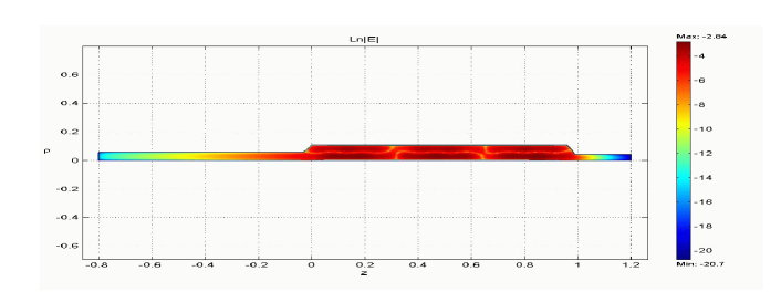
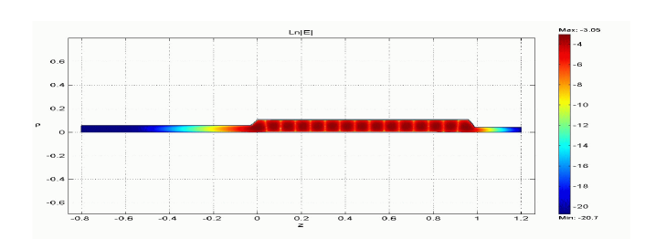
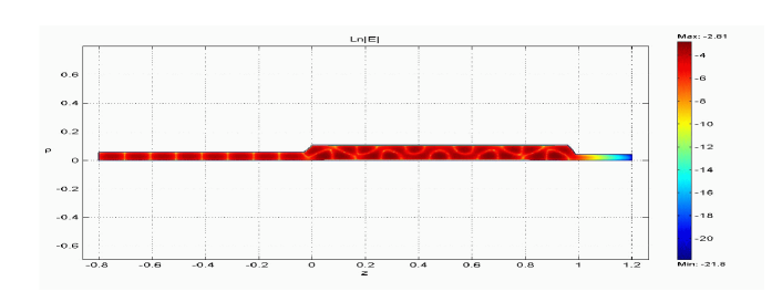
Figure 1: The geometry of the cavity and the mode structure for the filtering geometry. Note that only half of the cavity is shown, since the other half is redundant due to rotational symmetry of the cavity as well as the fields. The small region to the right is the entrance region, the large middle region is where the interaction takes place, and the region to the left is the filtering region. All modes have the electric field in the angular direction, i.e. $\mathbf{E}=E(\rho,z)\widehat{\mathbf{\varphi}}$. The variations of $\ln\left|E(\rho,z)\right|$ are shown in color code.
a) The mode structure of pump mode 1. The exponential decay in the region of small cross-section diminishes the amplitude by a factor $10^{-6}$ in the end of the filtered region.
b) The mode structure of pump mode 2. The exponential decay in the region of small cross-section diminishes the amplitude by a factor $10^{-8}$ in the end of the filtered region.
c) The mode structure of the excited mode. The amplitude is roughly the same in the region of interaction and in the filtered region.

References

- (1) W. Heisenberg and H. Euler, Z. Physik 98 714 (1936).
- (2) J. Schwinger, Phys. Rev. 82 664 (1951).
- (3) Z. Bialynicka–Birula and I. Bialynicki–Birula, Phys. Rev. D 2 2341 (1970).
- (4) M. Marklund, G. Brodin and L. Stenflo, Phys. Rev. Lett. 91 163601 (2003).
- (5) B. Eliasson and P.K. Shukla, Phys. Rev. Lett 92, In press.
- (6) R.L. Dewar, Phys. Rev. A 10 2017 (1974).
- (7) E.B. Alexandrov, A.A. Anselm and A.N. Moskalev, Zh. Eksp. Teor. Fiz. 89 1181 (1985) [engl. transl. Sov. Phys. JETP 62, 680 (1985))].
- (8) Y.J. Ding and A.E. Kaplan, Phys. Rev. Lett. 63 2725 (1989).
- (9) N.N. Rozanov, Zh. Eksp. Teor. Fiz. 103 1996 (1993) [engl. transl. Sov. Phys. JETP 76, 991 (1998)].
- (10) N.N. Rozanov, Zh. Eksp. Teor. Fiz. 113 513 (1998) [engl. transl. Sov. Phys. JETP 86, 284 (1998)].
- (11) Y.J. Ding and A.E. Kaplan, J. Nonlinear Opt. Phys. Mater. 1 51 (1992).
- (12) M. Soljacic and M. Segev, Phys. Rev. A 62 043817 (2000).
- (13) B. Shen, M.Y. Yu and X. Wang, Phys. Plasmas 10 4570 (2003).
- (14) A.E. Kaplan and Y.J. Ding, Phys. Rev. A, 62, 043805 (2000).
- (15) G. Brodin, M. Marklund and L. Stenflo, Phys. Rev. Lett. 87 171801 (2001).
- (16) S. Brattke, B.T.H. Varcoe and H. Walther, Phys. Rev. Lett. 86 3534 (2001).
- (17) G. Nogues et al., Nature 400 239 (1999).
- (18) Note that the characteristic field is related to the critical field that puts the limit of validity for the Euler-Heisenberg Lagrangian through .
- (19) J. Graber, Ph.D. Dissertation (Cornell University, 1993)
- (20) K. Saito, Critical field limitation of the niobium superconducting RF cavity, SRF 2001 conference proceedings, see http://conference.kek.jp/SRF2001/pdf/PH003.pdf
- (21) M. Liepe, eConf C00082 WE204, (2000), see also Pulsed Superconductivity Acceleration, http://xxx.lanl.gov/physics/0009098