Scaling and singularity characteristics of solar wind and magnetospheric fluctuations

Abstract

Preliminary results are presented which suggest that scaling and singularity characteristics of solar wind and ground based magnetic fluctuations appear to be a significant component in the solar wind - magnetosphere interaction processes. Of key importance is the intermittence of the ”magnetic turbulence” as seen in ground based and solar wind magnetic data. The methods used in this paper (estimation of flatness and multifractal spectra) are commonly used in the studies of fluid or MHD turbulence. The results show that single observatory characteristics of magnetic fluctuations are different from those of the multi-observatory AE-index. In both data sets, however, the influence of the solar wind fluctuations is recognizable. The correlation between the scaling/singularity features of solar wind magnetic fluctuations and the corresponding geomagnetic response is demonstrated in a number of cases. The results are also discussed in terms of patchy reconnection processes in magnetopause and forced or/and self-organized criticality (F/SOC) of internal magnetosphere dynamics.

1 Introduction

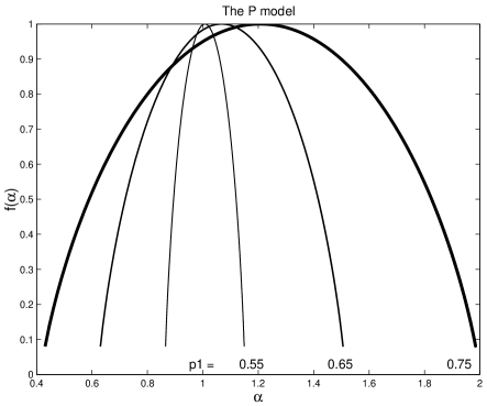
Figure 1: The $P$-model for three different values of parameter $p_{1}$

According to recent knowledge magnetospheric plasma fluctuations may be explained in terms of multiscale intermittent models including nonlinear self-organization processes (forced or not) near criticality (F/SOC) [Chang(1992), Chang(1999), Chapman et al.(1998), Takalo et al.(1999), Klimas et al.(2000)]. The basic physical concepts and the corresponding path-integral and renormalization group formalisms of nonlinear self-organization of magnetospheric processes are described in [Chang(1999)]. These models predict multifractality, non-Gaussian, power-law distributions for certain measurable physical quantities and associated power-law scalings for power spectra. In fact, several experimental studies seem to support the theoretical predictions quite well [Consolini et al.(1996), Milovanov et al.(1996), Consolini(1997), Borovsky et al.(1997), Consolini and De Michelis(1998), Vörös (1998), Uritsky and Pudovkin (1998), Consolini and Lui(1999), Chapman et al.(1999), Freeman et al.(2000a), Freeman et al.(2000b), Sharma et al.(2001)]. Scale-free power spectra of magnetospheric fluctuations, however, admit several possible explanations other than F/SOC. [Watkins et al.(2001a)] compared linear noisy, low-dimensional nonlinear, stochastic fractional Brownian motion (fBm) and SOC models of magnetospheric fluctuations to examine their scaling and predictabilitity properties. They concluded that the SOC model is of particular interest to magnetospheric physics due to its robustness in explaining scalings under the wide range of activity levels exhibited by the magnetosphere and the solar wind. On the other hand, weakly nonlinear models with fBm type noise added could explain the scaling and predictabitity properties of magnetospheric fluctuations equally well. Geomagnetic fluctuations on the time scale of substorms and storms certainly appear to be a compound mixture of multiscale magnetospheric processes including the component represented by intermittent solar wind fluctuations [Chang(1999), Daglis et al.(1999)]. Spectral methods making a distinction between these constituents may be queried to a certain extent mainly because the information on nonlinear multiscale structures is partially hidden for second order statistics. For example, [Tsurutani et al.(1990)] using the AE-index time series have shown that the power spectrum of the AE data exhibits two different power law scalings divided by a spectral break at the frequency range about 1/(5h). While the higher frequency part was thought to be more intrinsic to the magnetosphere, the lower frequency part was attributed to the influence of solar wind. [Vörös(2000)] has shown that similar results can be obtained also by means of a multifractal technique, which also makes possible, however, to reveal additional information on singularity distributions of high-latitude geomagnetic fluctuations (see later), not evident from spectral studies. Among other things, the results of multifractal analysis show that the local singularity (Hölder) exponents are time dependent and the previously proposed fBm type or bicolored noise model [Takalo et al.(1993)] of geomagnetic fluctuations is not relevant. Moreover, for a range of singularity exponents, a multiplicative cascade model, (the $P$-model) describes quite well the observed singularity distribution of geomagnetic fluctuations. Out of this range, however, significant deviations from a multiplicative model appear. The $P$-model describes energy cascade processes in turbulent flows. The largest turbulent eddy is assumed to be built up by a specific energy flux per unit length. Then a scale-independent space-averaged cascade-rate is considered and the flux density is transferred to the two smaller eddies with the same length but different flux probabilities $p_{1}$ and $p_{2}$. This process with randomly distributed $p_{1}$ and $p_{2}$ ($p_{1}$ + $p_{2}$ = 1) is repeated towards smaller and smaller scales. Energy transfer rate is homogeneous for $p$ = $p_{1}$ = $p_{2}$ = 0.5 while $p_{1}$ $>$ 0.5 corresponds to an intermittent flow. Figure 1 shows how the intermittence increases with increasing parameter $p_{1}$ [Tu et al.(1996)] in $\alpha$, $f(\alpha)$ plane [Halsey et al.(1986)]. The larger spread of $\alpha$ values around right-shifted $\bar{\alpha}$, the more intermittent field. In spite of the simplicity of the outlined cascade model its relevance for the description of intermittence effects in magnetospheric fluctuations may lead to the assumption that turbulence rather than F/SOC models fit the observed statistics better. Some results on statistical distribution of internal time periods between bursty geomagnetic events (waiting times) [Kovács et al.(2001)] seem to support this assumption. SOC models (at least the original [Bak et al.(1987)] model) are expected to display an exponential waiting time distribution. Geomagnetic data, however, display a well-defined power-law waiting time distribution. It was pointed out by [Boffetta et al.(1999)] that the observed power-law waiting time statistics in solar flares appears to be well explained by MHD shell models of turbulence. Similar results were presented by [Spada et al.(2001)] who analysed density fluctuations in a magnetically confined plasma system and found that waiting time statistics is in contrast with the predictions of an SOC system. An opposite view was presented by [Freeman et al.(2000b)] who conjectured that a wider class of running sandpile models [Hwa and Kardar(1992)] could exhibit power law behaviour in the probability density functions of waiting times. [Watkins et al.(2001b)] determined that the PDFs for burst durations and waiting times in a reduced MHD simulation follow power-laws which is not sufficient to distinguish between turbulence, SOC-like models and colored noise sources. [Boffetta et al.(1999)] and [Antoni et al.(2001)] also argued that SOC models represent self-similar, fractal phenomena. Geomagnetic fluctuations exhibit clear multifractal scaling [Consolini et al.(1996), Vörös(2000)] which seems to contradict to SOC concepts again. [Georgoulis et al.(1995)], however, demonstrated that the SOC state displayed by their cellular automaton model of isotropic and anisotropic energy avalanches has multifractal and multiscaling characteristics, rather than single power-law scalings and this feature was even enhanced by considering extended instability criteria. Similar SOC models of solar flares also exhibit multifractal and multiscaling characteristics [Vlahos et al.(1995)]. Recent works [Vassiliadis et al.(1998), Isliker et al.(1998), Isliker et al.(2000), Georgoulis et al.(2001), Uritsky et al.(2001)] underline the proximity between the SOC rules and laws of MHD in space physics systems, which are long known to exhibit turbulent behaviour (Georgoulis, personal communication, 2001). More realistic F/SOC models which include e.g. less artificial feedback mechanisms, a wide variety of drivings, interacting avalanches, SOC in continuum physical systems [Lu (1995)], etc. may further establish the proximity with turbulence. As pointed out by [Uritsky et al.(2001), b] the concept of SOC in a continuum limit (fluid or MHD limit) is essentially unexplored. [Klimas et al.(2000)] proposed a simplified Earth’s magnetotail current sheet model based on continuum SOC model of [Lu (1995)]. The continuum Lu model in a magnetic field reversal configuration can evolve into SOC due to localized rapid magnetic field annihilation within the field reversal region. In the same time, the plasma sheet is dominated by strong turbulence which keeps the system near criticality and produces a predictable quasi-periodic loading-unloading cycle of coherent global substorm activity [Klimas et al.(2000)]. In this model turbulence, SOC states and coherent global modes coexist within the Earth’s magnetotail on different scales. As a result, the observed ground based and satellite time-series contain a mix of fluctuations of different physical origin. [Angelopoulos et al.(1999)] further argued that the presence of intermittent turbulence in the Earth’s magnetotail may alter the conductivity and the mass/momentum diffusion properties across the plasma sheet and may permit cross-scale coupling processes playing also an important role in the establishment of SOC state.

In this paper no attempt will be made to participate in the theoretical debate on SOC or turbulence. However, having a pragmatic view, our opinion is that measures of intermittence or characteristic descriptors of cascade processes, commonly used in turbulence studies, like the flatness and multifractal spectra, could be applied in solar wind-magnetosphere interaction studies for further comparison of basic characteristics of intermittent fluctuations in solar wind and within the magnetosphere. We assume this aproach might be useful providing experimental information on such characteristics of fluctuations which are not accessible for spectral studies or second order statistics. This assumption was already investigated in [Vörös (1998), Vörös(2000), Vörös and Kovács(2001), Kovács et al.(2001)]. The preliminary results allow to make a working hypothesis that intermittence, scaling, rapid changes, singularities represent an essential piece of information regarding the effectiveness of SW - magnetosphere coupling not considered enough hitherto. In order to go deeper, we analyse different geomagnetic and solar wind data sets and make a comparison between various magnetic activity levels considering time scales of geomagnetic storms (from hours to days), substorms (from half an hour to a few hours) or less.

The main goal of this comparative study is to contribute to the understanding of solar wind - magnetosphere interaction processes on the basis of characteristic scaling/singularity features of the considered time series. We recall that solar wind (SW) fluctuations are strongly intermittent [Burlaga(1991)], that is energy at a given scale is not homogeneously distributed in space or/and time. Several studies on characteristic probability distribution functions (PDF) of increments of SW parameters (magnetic field, velocity, temperature, Elsässer variable, etc.) [Marsch and Tu(1994), Sorriso-Valvo et al.(1999)] and on multifractal structure of SW fluctuations [Burlaga(1992), Carbone(1994), Marsch et al.(1996), Tu et al.(1996)] support this assumption. Moreover, [Veltri and Mangeney(1999)] and [Bruno et al.(1999)] have shown that there is a direct link between intermittence and the presence of SW structures (Alfvénic, magnetic fluctuations, discontinuities) across which the magnetic field magnitude changes. Also, the high frequency (small scale) fluctuations of the southward component of the interplanetary magnetic field have a different spectral scaling exponent as the one exhibited by geomagnetic AE index fluctuations. On larger scales the corresponding spectra are similar [Tsurutani et al.(1990)]. A comparative study of dynamical critical scalings in the auroral electrojet (AE) index versus solar wind fluctuations confirmed that for times shorter than 3.5 hours (higher frequencies) the AE index fluctuations are of internal magnetospheric origin [Uritsky et al.(2001)].

2 Data analysis methods

As usual, we introduce the concept of scale ($\tau$) through the difference

$$\delta X(t,\tau)=X(t+\tau)-X(t)$$ (1)

where $X(t)$ is the time series under consideration. [Marsch and Tu(1994)] have shown that the PDFs of the increments $\delta X$ ($X$ - SW parameters) exhibit strong deviations from Gaussianity, especially at smaller scales and the effect is due to intermittence of SW fluctuations. To quantify the degree of deviation from the Gaussian distribution, i.e. the level of intermittence at different scales, we compute the flatness defined by

$$F=\frac{<\delta X(t,\tau)^{4}>}{<\delta X(t,\tau)^{2}>^{2}}$$ (2)

The flatness of a normally distributed signal is equal 3. Adding intermittent fluctuations to an originally Gaussian signal implies the spreading of its PDF, and consequently, the increase of its flatness from the original value of 3.

Non-homogeneous/intermittent distributions in space/time may also appear as asymptotically singular and can be characterized locally, at the point $t_{i}$, by the singularity (Hölder) exponents $\alpha$ as [Véhel(1996), Véhel and Vojak(1998), Riedi(1995), Canus(1998)]

$$\alpha_{n}^{k}(t_{i})=\lim_{n\rightarrow\infty}\frac{-log\mu(I_{n}^{k}(t_{i}))}{n}$$ (3)

where $\mu$ is a measure constructed from a time series. The procedure involvs the computation of the energy content of the differenced signal (Eq. 1) by taking its squared value. The measure at a point $t_{i}$ is given by $\delta X^{2}(t_{i},\tau)/\sum_{i}\delta X^{2}(t_{i},\tau)$. To analyse the distribution of singularity exponents (Eq. 3) a sequence of partitions $P$ is introduced so that [Véhel(1996)]

$$P_{n}=\{I_{n}^{k}\};\>\>\>\>\>\>\>\>0\leq k<2^{n}-1$$

$$I_{n}^{k}=<k2^{-n},(k+1)2^{-n})$$

where $I_{n}^{k}$ is the interval containing t and the resolution is set by $n$. The quantity of interest is the so-called large deviation singularity spectrum, $f(\alpha)$, which represents a rate function measuring the deviation of the observed $\alpha$ from the expected value $\overline{\alpha}$. The rate function, $f(\alpha)$, can be estimated through [Véhel(1996)] :

$$f(\alpha)=\lim_{n\rightarrow\infty}\frac{N_{n}(\alpha)}{n}$$ (4)

where $N_{n}(\alpha)$ is the observed number of coarse grain Hölder exponents . Usually ”histogram methods” for estimation of $f(\alpha)$ are used. In that case the number of those intervals $I_{n}^{k}$ for which $\alpha_{n}^{k}$ falls in a box between $\alpha_{min}$ and $\alpha_{max}$ is computed and $f(\alpha)$ is found by a regression. It yields satisfactory results for pure multiplicative processes, but fails to describe non pure or compound processes when $f(\alpha)$ is not a concave function. To overcome this difficulty the so-called double kernel method was proposed [Véhel(1996), Véhel and Vojak(1998)] realizing that $N_{n}(\alpha)$ may be written as a convolution of the density of the $\alpha_{n}^{k}$s and a compactly supported kernel. This method allows to estimate non concave rate functions and we are going to show that this property may be properly used for characterization of fluctuation processes in near-Earth space. In this paper the estimations of $f(\alpha)$ spectra were realized using the FRACLAB package developed at the Institut National de Recherche en Informatique, Le Chesnay, France.

3 Ground based data

In order to study the basic characteristics of auroral zone geomagnetic fluctuations we analyse geomagnetic $H$-component 1-min mean data from polar cap observatory, THULE (THL: $77.47^{o}$ N, $290.77^{o}$ E), geomagnetic $X$-component 1-min mean data from high-latitude observatory NARSSARSSUAQ (NAQ: $61.16^{o}$ N, $314.57^{o}$ E) and 1-min mean auroral electrojet (AE) index time series, all from 1991-1992.

As known, the AE-index was introduced by [Davis and Sugiura(1966)] to describe the global activity of the auroral zone electric currents and is derived, after the substraction of base line values, from evaluation of the variations measured at 12 stations located near the northern auroral zone. There exist a large number of physical mechanisms which couple the auroral zone processes with those within magnetospheric tail or in SW. Recently, intermittent energy transport in the magnetotail, the so called bursty bulk flow events (BBF) came into the limelight of the magnetosphere research [Baumjohann(1990), Angelopoulos et al.(1992)]. From this point of view the understanding of the response of auroral zone currents or dissipation fields to the time - varying magnetotail dynamics seems to be important. There was not full understanding achieved regarding the nature and origin of the related magnetic fluctuations. Partly it was already explained in the introduction that it is related to the paradigms of F/SOC versus turbulence. We mention here some other open questions. For example it was shown that the burst lifetime distributions of some SW parameters are also of power law form, which might be a signature of SOC or turbulence regimes in SW [Freeman et al.(2000a), Kovács and Vörös (2001)]. Therefore, it is supposed that the scale free property of the AE-index may arise from the SW input or at least the internal dynamics of the magnetosphere may be masked by the scale free properties of SW driver [Freeman et al.(2000a)]. Again we remind, however, the very limitations of second order statistics in interpretation of the observed scalings. Another measure of the auroral zone dissipation fields is represented by polar optical activity within UVI bands. [Lui et al.(2000)] have examined the blobs of brightness as a proxy for BBF events. It was found that the non-substorm ”internal” events have a power law distribution whereas the system wide events like substorms besides a scale free region exhibit a ”bump”, corresponding to a mean value in substorm breakups. A somewhat opposite view was presented by [Consolini and De Michelis(1998)] who analysed AE-index fluctuations on time scales 1-120 [min] both in quiet (laminar phase) and disturbed periods (turbulent phase). They found that in both phases the intermittence at different time scales rescales in the same way and the non-Gaussian character of PDFs seems to be due to the same physical processes.

Here we pose the question again about the scaling and singularity properties of the AE-index, compared to the similar characteristics of geomagnetic data from two observatories THL and NAQ. As the AE index is derived from geomagnetic variations in the horizontal component observed at selected observatories along the auroral zone in the northern hemisphere, we expect that the scale $\tau$ (Eq. 1) cannot be precisely defined. The geographic distance between observatories through Taylor’s hypothesis already introduces some effective time shift (scale, $\tau$). Though, the application of the Taylor hypothesis within the magnetosphere is limited [Dudok de Wit and Krasnoselskikh (1990)]. Besides, from the recordings of auroral stations the greatest (upper envelope) and smallest (lower envelope) values are taken at intervals of one minute and their difference defines the AE-index. As far as the contributing observatory which gives the lower/upper envelope changes during the times, and the fluctuations with values between the upper and lower envelopes are not taken into account at all (smoothing), the AE-index appears to be a measure of auroral zone processes with mixed scales. This is certainly not an advantage when a multiscale analysis of AE-index time series is performed. This fact is usually neglected in the related literature. A less sophisticated way is to take data from a single observatory, but it may have some other drawbacks because significant distant disturbance events can be missed. Also, some BBFs with short duration may remain undetected on the ground because of their localized nature [Daglis et al.(1999)]. Nevertheless, a comparison of fluctuations of the ”multi-observatory measure” (MOM: AE-index) and of the ”single observatory measure” (SOM: THL geomagnetic field $H$-component and NAQ geomagnetic field $X$-component) may be instructive.

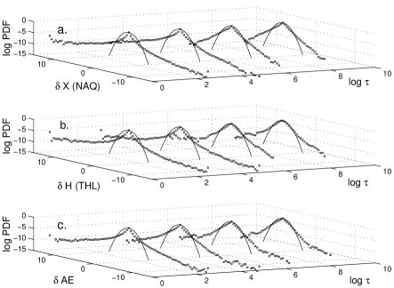
Figure 2: Probability distribution functions computed for: a. NARSSARSSUAQ $X$-component geomagnetic field; b. THULE $H$-component geomagnetic field; c. AE-index data. The time scales are $\tau=5,50,500,5000$ [min]. Continuous lines refer to Gaussian distribution, while the ”o” markers correspond to the analysed data.

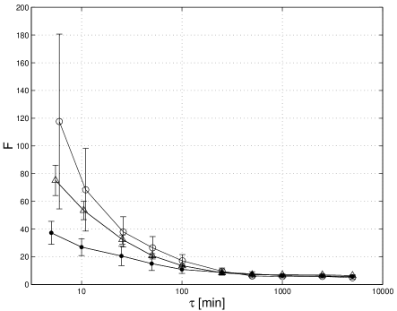
Figure 3: The flatness as a function of scale ($\tau\in(5,5000)$ [min]) estimated for NARSSARSSUAQ ($\bigtriangleup$), THULE data (o) and AE-index ($\bullet$).

Figure 2 shows the PDFs from normalized increments $\delta X$ (Eq.1) of the SOM (Figure 1a, b) and MOM (Figure 1b) data (X $\equiv$ X(NAQ), H(THL) and AE, respectively). Calculations have been made for $\tau$ = 5, 50, 500, 5000 [min] and 1 minute mean data was considered from the years 1991-1992. As can be seen the distributions in all cases change with $\tau$, and for smaller values of $\tau$ significant deviations from the normal distribution occur. The tails of the distributions reduce with increasing scale parameter as a consequence of the decrease of the probability of coherent fluctuations between points separated by increasing distance. The difference between the MOM and SOM is more clear if the flatness ($F$) of the corresponding distributions is compared (Eq. 2). Figure 3 shows how the flatness evolves with increasing $\tau$ ($\tau$ $\in$ (5, 5000) [min]). The errorbars correspond to the standard deviations (std) computed from time series divided to several parts. For small scales, say, $\tau$ less than a few tens of minutes, the AE-index (MOM) exhibits smaller deviations from the normal distribution than NAQ (SOM). $F(NAQ)$ reaches the level of $F_{max}$ (AE, $\tau$ = 5) only at the value $\tau$ $\sim$ 30 [min], which roughly may be considered as the effective time shift introduced by the method of derivation of the AE-index. THL (polar cap observatory) data essentially show the same behaviour as NAQ, but the stds are larger. Therefore, we conjecture that MOMs (multi-observatory geomagnetic indices), due to smoothing and scale mixing effects, lead to underestimation of the intermittence on small scales. Henceforth, we will show only the dependence of the flatness on scale parameter $\tau$.

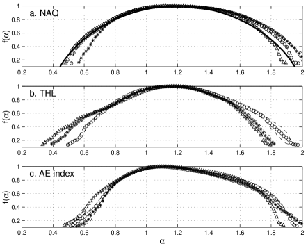
Figure 4: Dependence of singularity rate functions on scale; $\tau=5(\bigtriangleup);50(\ast);500(o)$ [min]. a. NARSSARSSUAQ data, b. THULE data; c. AE-index. Thick line in Figure 4a corresponds to $P$-model fit.

Let us consider now the singularity distributions $f(\alpha)$ (Eq. 3, 4) for the same data sets as above. To see better how the $f(\alpha)$ rate functions evolve with $\tau$, all the curves are depicted at the same plane $(\alpha,f(\alpha))$ in Figure 4. Proper symbols are introduced for the scales $\tau$ = 10, 50, 500 [min] ($\bigtriangleup,*,o$) and the dashed lines correspond to the errors estimated by changing the resolution in Eq. 3, 4. (No averaging needs to be done estimating $f(\alpha)$ [Véhel(1996)] so the spectrum may be evaluated at only one resolution. However, to show that the estimations are consistent, all the spectra were computed using 15 different resolutions). Again, there are several differencies between the SOM and MOM data. Figure 4a shows the singularity spectra for NAQ observatory data. On the considered scales, the shape of the curves is almost parabolic, close to the $P$-model fit (thick curve) with $p_{1}\sim 0.745$. The best correspondence is achieved for the smallest value of $\tau$ = 10 [min] (depicted by symbol $\bigtriangleup$ on Figure 4a). It means that in case of auroral zone SOM fluctuations and especially on small scales, the deviations from the Gaussian distribution (Figure 3) can be explained by a simple cascade model. Though the phenomenology of turbulent cascades in fluid flows is more complex than the simple $P$-model fit in Figure 4a would lead us to indicate, the 1D cascade model rouhgly describes how the auroral zone SOM fluctuations become more and more intermittent at smaller and smaller scales. The spectra for polar cap (THL observatory) SOM (Figure 4b) and AE index MOM (Figure 4c) have a more pronounced non-parabolic shape indicating the presence of compound processes. At small scales ($\tau$ = 5,50 [min]) THL observatory fluctuations contain stronger singularities because of the extension of the rate functions left wings to the smaller (more singular) values of $\alpha$. For $\tau$ = 500 [min], however, the right wing evolves to the less singular values which may be related to the SW influence [Vörös(2000)]. This effect is less visible, but still present in auroral zone SOM data (Figure 4a). The MOM AE index $f(\alpha)$ spectra practically do not change with $\tau$. We conjecture, this is the result of the method of derivation of the AE index, resulting smoothing and scale mixing effects.

In all cases, the deviations of singularity spectra from the parabolic shape may be indicative of the phenomenon of phase transition. Namely, at the $\alpha$ values where the $f(\alpha)$ spectra are out of parabolic shape the major contributor to the observed singularities may change from one measure to another. As different physical processes may generate different measures (distributions), possible models with similar characteristics as the observed spectra may contain physical information on the contributing (e.g. SW or magnetospheric) sources.

4 Satellite data

The very advantage of the ground based data is its availability for a long periods of time. For a proper estimation of PDFs or singularity rate functions long data sets are needed which is a requirement hardly ever fulfilled in the case of satellite data. Nevertheless, we expect to find out some interesting scaling/singularity features of interplanetary magnetic field (IMF) fluctuations proceeding in the same way as in the previous section. To this end we analyse ACE and WIND IMF $B$ magnitude and $B_{z}$ component data which are available with time resolution of 16 [s] and 3 [s], respectively. SW velocity is not considered here due to too many gaps in data. While the ACE satellite is continuously monitoring the SW at the $L_{1}$ point, WIND has a more complicated trajectory crossing also the magnetosphere from time to time. For our analysis we have chosen time periods when WIND was also in SW and there were negligible data gaps in both cases (less than 1 $\%$ of total data lengths).

Another aim was to analyse ”geoeffectively different” periods of IMF $B$ and $B_{z}$ magnitude fluctuations. Geoeffectiveness during the chosen periods was considered examining the geomagnetic $D_{st}$ index which is derived from the geomagnetic field $H$-component registrations of 4 observatories [Sugiura(1964)] and it aims at giving the effect of the magnetospheric ring currents. The chosen periods were classified as disturbed ones if geomagnetic fluctuations with storm-index $D_{st}$ being less than -50 [nT] occured several times within a consedered interval. The limit of $D_{st}<$ -100 [nT] which corresponds to intense storms was considered, too. We emphasize, however, instead of a study of individual storms, the generic features of fluctuations on a given scale $\tau$, but during longer periods of time are investigated. Essentially 2 $\div$ 4 weeks of data with the consedered time resolutions may already ensure sufficiently robust estimations of singularity spectra (Eq. 4). In this sense, several intense magnetic storms $D_{st}$ $\ll$ -50 [nT] may occur during a strongly disturbed interval, a less disturbed period contains less intense storms and an undisturbed period has only $D_{st}>$ -50 [nT]. The limit of -50 [nT] was chosen on the basis of previous studies of magnetic storms [Taylor et al.(1996)]. Intense magnetic storms are characterised by $D_{st}$ index $<$ -100 [nT] [Gonzalez and Tsurutani(1987)]. In this preliminary study of generic features of magnetic fluctuations these limits may be consedered as more or less adequate. We expect that this rough classification of the geomagnetic response allows us to identify characteristic scaling and singularity features of the corresponding IMF magnetic fluctuations that would be indicative for their geoeffectiveness.

There were 5 time periods and 6 data sets separated for our analysis (for one period there were both ACE and WIND data available). The disturbed periods are the following: $1.$ March 19 - April 25, 2001 (ACE); $2.$ October 1 - November 30, 2000 (ACE); $3.$ April 9 - April 20, 1997 (WIND). The undisturbed periods: $4.$ November 18 - December 10, 1998 (ACE); $5.$ January 10 - January 29, 1998 (ACE, WIND). For demonstration we show some of the data sets.

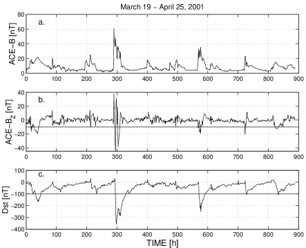
Figure 5: An extremely disturbed period as seen in 1-hour mean a. ACE IMF magnitude, b. ACE IMF $B_{z}$ component and c. $D_{st}$-index data plots.

Figure 5 shows the first ACE data set from March 19 to April 25, 2001. For the sake of perspicuity, the time resolution is 1 [h]. (The flatness and singularity spectra are computed from the time series with time resolution of 16 [s] and 3 [s].) During this extremely active period intense magnetic storms ($D_{st}$ $\leq$ -100 [nT]) occured several times (Figure 5c). The limit of -100 [nT] is depicted by a thick line in Figure 5c. [Gonzalez and Tsurutani(1987)] have shown that the interplanetary causes of intense magnetic storms are long duration ($>$ 3 [h]), large and negative ($<$ -10 [nT]) IMF $B_{z}$ events associated with interplanetary duskward electric fields $>$ 5 [$mVm^{-1}$]. In Figure 5b IMF $B_{z}$ is depicted, including a thick line indicating the level of -10 [nT]. Comparison of Figures 5b, c shows an agreement with the above criteria, that is, long duration negative IMF $B_{z}$ events occur together with intense magnetic storms. Figure 5a shows the variations of IMF $B$. It is visible that an intense magnetic storm occured at the end of the studied period, between $t$ = 800 and 900 [h] (Figure 5c). $B_{z}<$ 10 [nT] (Figure 5b) and $B_{max}\sim$ 17 [nT] corresponded to this event. A similar enhancement of $B$ at 400 [h] $\leq$ $t$ $<$ 450 [h] appears in Figure 5a having no intense storm response in $D_{st}$, which can be explained by the corresponding IMF $B_{z}>$ -10 [nT] in Figure 5b.

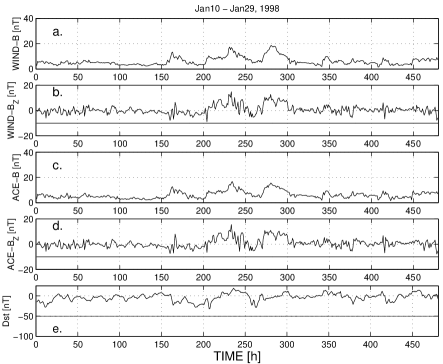
Figure 6: Undisturbed period as seen in 1-hour mean a. IMF $B$ (WIND); b. IMF $B_{z}$ (WIND); c. IMF $B$ (ACE); d. IMF $B_{z}$ (ACE) data plots and e. the corresponding geomagnetic response represented by $D_{st}$-index.

Figure 6 shows an undisturbed period from January 10 to January 29, 1998. Again, IMF $B$, $B_{z}$ (WIND, ACE Figures 6a-d) and $D_{st}$ index (Figure 6e) are shown. It is visible that $D_{st}>$ -50 [nT] and $B_{z}>$ -10 [nT] everywhere.

Fluctuations of IMF and their geoeffectiveness were studied by a number of authors. [McPherron et al.(1986)] showed that substorms are frequently triggered by changes in the IMF. [Kamide(2001)] proposed that the quasi-steady component of the interplanetary electric field is imporant in enhancing the ring current, while its fluctuations are responsible for initiating magneospheric substorms. It is out of scope of this paper to analyse the influence of other interplanetary parameters (e.g. velocity, density, temperature, etc.) on storm/ substorm activity [Daglis et al.(2001)]. Rather we will concentrate on the level of intermittence of IMF fluctuations.

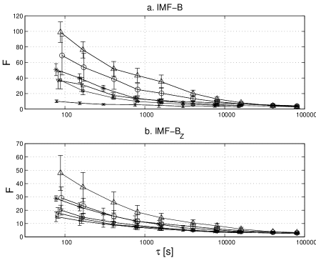
Figure 7: The flatness as a function of scale ($\tau\in(16*5,16*10^{5})$ [sec]) estimated for the periods: March 19 - April 25, 2001, (ACE: $\bigtriangleup$); October 01 - November 30, 2000, (ACE: o); April 09 - April 20, 1997, (WIND: $\ast$); November 18 - December 10, 1998, (ACE: $\bigtriangledown$); January 10 - January 29, 1998, (WIND: x); January 10 - January 29, 1998, (ACE: $\diamond$). Disturbed, that is geoeffective events are depicted by larger markersizes. a. IMF $B$, b. IMF $B_{z}$.

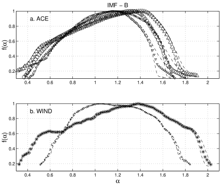
Figure 8: Singularity spectra (rate functions) estimated for IMF $B$. The periods and data sets are depicted by the same marker types as in Figure 7.

To this end let us consider the flatnesses and the singularity rate functions for the disturbed and undisturbed periods of $1-5$. Deviations from the Gaussian distribution are larger in the case of disturbed events depicted by larger markersizes in Figure 7. The PDFs of the undisturbed events are also non-Gaussian, but the flatnesses for a given scale are smaller than those for disturbed events especially at scales $\tau<$ 1000 [s]. Similar differences are present in singularity spectra computed for IMF $B$ fluctuations at the scales of $\tau$ = 320 [sec] (ACE) and $\tau$ = 60 [s] (WIND) shown in Figure 8. There were the same marker types used as in Figure 7. ACE and WIND data are depicted separately in Figures 8a, b. The maxima of the singularity spectra of more disturbed periods have a tendency for shifting to larger values of $\alpha$. Also, the spread of singularities around most probable $\alpha$ is wider for more disturbed cases. But it is the same behaviour as in case of the simple $P$-model in Figure 1, when intermittence is stronger and stronger for larger and larger values of $p_{1}$. The differences between the disturbed and undisturbed cases gradually cease for larger values of $\tau$ (not shown).

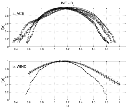
Figure 9: Singularity spectra estimated for IMF $B_{z}$. The periods and data sets are depicted by the same marker types as in Figure 7.

Figure 9 shows the singularity spectra computed for IMF $B_{z}$ fluctuations in the same way as previously. Obviously, the intermittent fluctuations of IMF $B$ and $B_{z}$ fields exhibit very similar changes in their flatnesses and singularity spectra as the geoeffectivity level changes. For example, there is a clear difference between the introduced scaling and singularity characteristics (Figure 5) for the disturbed period March 19 - April 25, 2001 and for the undisturbed period January 10 - January 29, 1998 (Figure 6). It indicates that, in addition to known ”geoeffective” SW parameters (e.g. southward component of IMF) or their combinations, small scale rapid changes, singularities and non-Gaussian statistics of IMF fluctuations may play an important role in SW - magnetosphere interaction processes.

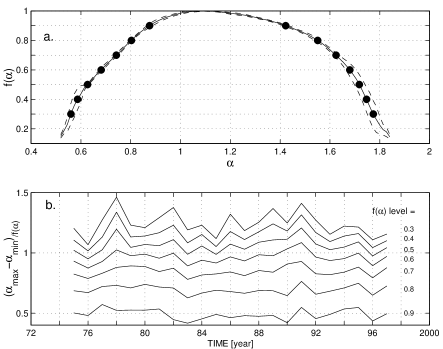
Figure 10: Time variation of the shape of singularity spectra a. filled circles show the points in which $\alpha_{min}$ and $\alpha_{max}$ values are computed; b. $\alpha_{max}-\alpha_{min}$ values computed at different $f(\alpha)$ levels.

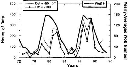
Figure 11: Yearly averaged number of hours with $D_{st}$ $<$ -100 nT ($\diamond$), and with $D_{st}$ $<$ -50 nT ($-\>-\>-$). Yearly averaged sunspot number (thick line) is also shown. After [Kamide et al.(1998)].

Also, the question naturally arises to what extent the magnetospheric response itself is influenced by small scale statistics of IMF fluctuations. Unfortunately, not all the geomagnetic data is available for the above analysed periods. It is possible to test, however, how the shape of the rate function changes if available data is considered. Minute-mean $H$-component geomagnetic data from THL observatory is available from 1975 to 1996. We computed the $f(\alpha)$ spectra for each year at the scale $\tau$ = 50 [min] and analysed how their shapes change at the $f(\alpha)$ values 0.3 - 0.9. At each level of $f(\alpha)$ the corresponding values of $\alpha_{min}$ and $\alpha_{max}$ were computed (filled circles in Figure 10a). In Figure 10b the time evolution of the difference $\alpha_{max}-\alpha_{min}$ at a given $f(\alpha)$ level is depicted. The average standard deviation at $f(\alpha)$ = 0.3 is about 0.06, while at $f(\alpha)$ = 0.9 is 0.02. At $f(\alpha)$ = 0.3 - 0.6 the $\alpha_{max}-\alpha_{min}$ curves strongly fluctuate indicating significant changes in the shape of $f(\alpha)$ spectra from 1975 to 1996. Figure 11 shows the similar results of [Kamide et al.(1998)], however, obtained by a different method. [Kamide et al.(1998)] analysed the occurence of geomagnetic storms in comparison with yearly averaged Wolf sunspot number. Figure 11 shows the yearly averaged number of hours with $D_{st}$ less than -100 [nT] (solid line with filled diamonds), and with $D_{st}$ less than -50 [nT] (divided by 5, dashed line). Thick line corresponds to yearly averaged sunspot number. It is visible that the maxima of geomagnetic activity and of solar cycle do not coincide. During the declining phase of the solar cycle coronal holes emerge from polar regions of the Sun which are continuous sources of fast-speed plasma causing a peak in recurrent geomagnetic storms activity [Kamide et al.(1998), Kamide(2001)]. The similarity between the variability of rate function shapes for $f(\alpha)$ = 0.3 $\div$ 0.6 (Figure 10b) and yearly averaged number of hours with prescribed $D_{st}$ indices (Figure 11) is remarkable. This correspondence also supports our working assumption that the shape of $f(\alpha)$ rate function estimated using Eqs. 3, 4 [Véhel(1996), Véhel and Vojak(1998)] contains relevant physical information. We mention that available AE-index and NAQ observatory data lead to the same results. On the other hand, however, at $f(\alpha)$ = 0.7 - 0.9 the variations of $\alpha_{max}-\alpha_{min}$ versus time are negligible (Figure 10b).

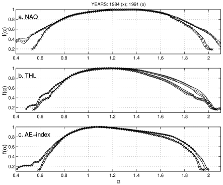
Figure 12: Singularity spectra for a. NARSSARSSUAQ data; b. THULE data; c. AE-index. Maximum of geomagnetic activity in 1991 (o); minimum of geomagnetic activity in 1984 (x).

On the basis of Figures 10b and 11, years with extreme levels of geomagnetic response can be chosen and their corresponding singularity spectra can be recalculated. Figures 12a-c show the SOM and MOM spectra estimated at $\tau$ = 50 [min] for maximum (1991, symbol o) and minimum (1984 - symbol x) years of geomagnetic activity. One can see that the characteristic asymmetric shape of AE-index spectra (Figure 12c) in comparison with Figure 4c is present henceforward, presumably caused by the influence of SW fluctuations. Noticeably, the maxima and the right wings of the more geoeffective SW IMF singularity distributions (Figures 8, 9) match well the region of $\alpha\in$ (1.2, 1.8) within which the MOM spectra for the most part are out of parabolic shapes. The same effect is visible for the more singular wing of $f(\alpha)$ spectra at $\alpha$ $\in$ (0.4, 0.8). The asymmetry is even enhanced in 1991 (maximum of geomagnetic activity). The differences between more active (1991) and less active (1984) years are present in SOM spectra mainly at the wings of $f(\alpha)$ rate function, too (Figures 12a, b). The most probable singularities around $\bar{\alpha}$ do not exhibit any changes.

5 Discussion

We presented an analysis of scaling and singularity characteristics of ground based and satellite magnetic fluctuations in this paper. These techniques are commonly used in studies of turbulent flows. As we oulined in the Introduction the supposed proximity between F/SOC and MHD turbulence models may allow to estimate measures of scaling, intermittence, etc., directly from time series, for futrher comparison aiming to help a development of tractable numerical models of highly variable SW - magnetosphere interaction (Georgoulis, personal communication, 2001). We think the results are not contradictory in this sense, but rather elucidate important aspects of magnetic field fluctuations which should be incorporated to more realistic F/SOC models of SW driven magnetospheric activity. Scaling and singularity characteristics of high-quality geomagnetic data from THULE and NARSSARSSUAQ observatories (Single Observatory Measures) and of AE-index (Multi Observatory Measure) were compared estimating PDFs, flatnesses and singularity rate functions. The same methods were applied for ACE and WIND data. The specific periods chosen for the analysis of SW fluctuations reflect the limited availability of high resolution satellite data for relatively longer periods of time. In spite of this, subgroups of disturbed and undisturbed periods were selected, having primarily in mind the occurence of enhanced geomagnetic response represented by 1-hour mean $D_{st}$-index. The comparison of generic features of fluctuations in SW and high-latitude SOM and MOM data is then possible, because geomagnetic activity at high-latitudes is always very high during magnetic storms, though the storm/substorm relationship itself is more complicated [Daglis et al.(2001)].

It was shown that the intermittence of AE-index fluctuations is reduced at small scales due to the method of its derivation. We argue this also provides a possible explanation for the negligible changes of the AE-index singularity distribution with $\tau$. Other kind of MOM data might be influenced in the same way. Nevertheless, the contribution of SW fluctuations make the AE-index rate function asymmetric, mainly within the range of $\alpha\in(1.2,1.8)$. The same asymmetry caused by the SW is also present in THL and NAQ rate functions, however, mainly for $\tau>300$ [min] (see also [Vörös(2000)]).

In case of SW fluctuations it was demonstrated that the departure from Gaussianity is stronger at small scales and it clearly depends on the correlation (geoeffectiveness) between IMF fluctuations and the occurence of geomagnetic storms (decreased $D_{st}$-index). It seems to indicate that the intermittence strength of IMF magnitude and $B_{z}$ component fluctuations, in addition to other SW parameters such as southward $B_{z}$, SW velocity, density, Alfvenic Mach number, plasma $\beta$, represents a new parameter (or rather a whole set of parameters describing singularity features) controlling the energy input rate to the magnetosphere. Considering Taylor’s hypothesis and SW velocities of 500 km/s, intermittence at time scales of tens of seconds corresponds to the spatial structures of several thousand kilometers or more. [Book and Sibeck(1995)] estimated the corresponding timescale on which turbulent motion may affect the transport of mass and energy across the magnetopause through interchange instability. They have found it is less than 150 [s]. As known from previous ISEE1 and 2 magnetometer studies dayside reconnection of IMF and GMF lines seems often to be a sporadic and patchy process and measurements obtained at and near the magnetopause indicate that reconnection does not necessarily occur across the all dayside magnetopause even under the favourable southward pointing IMF conditions [Rijnbeek et al.(1984)]. We conjecture, patchy reconnection may be related to intermittence and singularity characteristics of IMF turbulence at small scales. There is a number of works in which the role of turbulence in magnetopause reconnection processes is anticipated [Galeev et al.(1986), Drake et al.(1994), Kuznetsova and Roth(1995)]. We recall the work of [Galeev et al.(1986)] in which patchy reconnection was considered to be an irregular multiscale process associated with the magnetic field diffusion and self-consistently generated magnetic turbulence. Our results indicate that a number of singularity parameters (Hölder exponents) should be taken into account to properly describe the basic characteristics of the upstream SW turbulence. In this paper we examined the global distribution of IMF singularities and found clear differences between geoeffectively disturbed and undisturbed periods. Obviously, to understand better the role of turbulence in patchy magnetopause reconnection processes a proper time and space localization of IMF singularities will be needed.

As far as the magnetospheric response is considered, previous results [Vörös and Kovács(2001)] have suggested that global singularity spectra estimations of SOM and MOM data sets on different scales may allow to separate fluctuations of SW or magnetospheric origin. Our results show that the influence of the SW is perceptible mainly at the wings of the rate function, that is at smaller values of $f(\alpha)$. The most probable singularities ($f(\alpha)=0.8-1$) are less influenced by SW driver. Rate functions estimated for years 1975-1996 exhibit similar variations as geomagnetic activity studied by [Kamide et al.(1998)]. SW forcing effects were found when SOM and MOM singularity spectra for two years (1984 and 1991) of different geomagnetic activity levels were compared.

We believe that further development in this direction will result a better understanding of SW - magnetosphere interaction allowing more efficient prediction of space weather.

Acknowledgements The authors wish to acknowledge valuable discussions with Vincenzo Carbone, Giuseppe Consolini, Manolis Georgoulis, Alex Klimas, Nick Watkins, and Vadim Uritsky. We are grateful to Yohsuke Kamide and Ioannis Daglis for sending us their results. We acknowledge the use of the Fraclab package developed at the Institut National de Recherche en Informatique, Le Chesnay Cedex, France. Geomagnetic data from Thule observatory, Narssarssuaq observatory and AE-index as well as $D_{st}$-index data from WDC Kyoto are gratefully acknowledged. We are grateful to N. Ness (Bartol Research Institute) and R. Lepping (NASA/GSFC) for making the ACE and WIND data available. Z. Vörös and D. Jankovičová were supported by VEGA grant 2/6040. P. Kovács was supported by the Hungarian Science Research Fund (OTKA) under project number F030331 and by the Eötvös Scholarship provided by the Hungarian Scholarship Committee.

References

- [Angelopoulos et al.(1992)] Angelopoulos, V., Baumjohann, W., Kennel, C. F., Coroniti, F. V., Kivelson, M. G., Pellat, R., Walker, R. J., Luhr, H., and Paschmann, G., Bursty bulk flows in the inner central plasma sheet, J. Geophys. Res, 97, 4027–4039, 1992.
- [Angelopoulos et al.(1999)] Angelopoulos, V., Mukai, T., and Kokubun, S., Evidence for intermittency in Earth’s plasma sheet and implications for self-organized criticality, Phys. Plasmas, 6, 4161–4168, 1999.
- [Antoni et al.(2001)] Antoni, V., Carbone, V., Cavazzana, R., Regnoli, G., Vianello, N., Spada, E., Fattorini, L., Martines, E., Serianni, G., Spolaore, M., Tramontin, L., and Veltri, P., Transport processes in reversed-field-pinch plasmas: inconsistency with the self-organized criticality paradigm, Phys. Rev. Lett., 87, 045001-1-045001-4, 2001.
- [Bak et al.(1987)] Bak, P., Tang, C., and Wiesenfeld, K., Self-organized criticality: an explanation of 1/f noise, Phys. Rev. Lett., 33, 381–384, 1987.
- [Baumjohann(1990)] Baumjohann, W., Paschmann, G., and Luhr, H., Characteristics of high-speed ion flows in the plasma sheet, J. Geophys. Res, 95, 3801–3809, 1990.
- [Boffetta et al.(1999)] Boffetta, G., Carbone, V., Giouliani, P., Veltri, P., and Vulpiani, A., Power laws in solar flares: self-organized criticality or turbulence? Phys. Rev. Lett., 83, 4662–4665, 1999.
- [Book and Sibeck(1995)] Book, D. L., and Sibeck, D. G., Plasma transport through the magnetopause by turbulent interchange processes, J. Geophys. Res., 100, 9567–9573, 1995.
- [Borovsky et al.(1997)] Borovsky, J. E., Elphic, R. C., Funsten, H. O., and Thomsen, M. F., The Earth’s plasma sheet as a laboratory for flow turbulence in high-beta MHD, J. Plasma Phys., 57, 1–34, 1997.
- [Bruno et al.(1999)] Bruno, R., Bavassano, B., Pietropaolo, E., Carbone, V., and Veltri, P., Effects of intermittency on interplanetary velocity and magnetic field fluctuations anisotropy, Geophys. Res. Lett., 26, 3185–3188, 1999.
- [Burlaga(1991)] Burlaga, L. F., Intermittent turbulence in the solar wind, J. Geophys. Res, 96, 5847–5851, 1991.
- [Burlaga(1992)] Burlaga, L. F., Multifractal structure of the magnetic field and plasma in recurrent streams at 1 AU, J. Geophys. Res, 97, 4283–4293, 1992.
- [Canus(1998)] Canus, Ch., Robust large deviation multifractal estimation, Proc. Internat. Wavelets Conf., Tangier, 1998.
- [Carbone(1994)] Carbone, V., Scaling exponents of the velocity structure functions in the interplanetary medium, Ann. Geophys., 12, 585–590, 1994.
- [Chang(1992)] Chang, T., Low-dimensional behavior and symmetry-breaking of stochastic systems near criticality: Can these effects be observed in space and in the laboratory, IEEE Trans.Plasma Sci., 20, 691–694, 1992.
- [Chang(1999)] Chang, T., Self-organized criticality, multi-fractal spectra, sporadic localized reconnections and intermittent turbulence in the magnetotail, Phys. Plasmas, 6, 4137–4145, 1999.
- [Chapman et al.(1998)] Chapman, S. C., Watkins, N. W., Dendy, R. O., Helander, P., and G. Rowlands, A simple avalanche model as an analogue for magnetospheric activity, Geophys.Res.Lett., 25, 2397–2400, 1998.
- [Chapman et al.(1999)] Chapman, S. C., Dendy, R. O., and G. Rowlands, A sandpile model with dual scaling regimes for laboratory, space and astrophysical plasmas, Phys. Plasmas, 6, 4169, 1999.
- [Consolini et al.(1996)] Consolini, G., Marcucci, M. F., and Candidi, M., Multifractal structure of auroral electrojet index data, Phys. Rev. Lett., 76, 4082–4085, 1996.
- [Consolini(1997)] Consolini, G., Sandpile cellular automata and magnetospheric dynamics, in Cosmics Physics in the Year 2000, edited by S. Aiello et al., 123–126, Italy, 1997.
- [Consolini and De Michelis(1998)] Consolini, G., and De Michelis, P., Non-Gaussian distribution function of AE-index fluctuations: Evidence for time intermittency, Geophys. Res. Lett., 25, 4087–4090, 1998.
- [Consolini and Lui(1999)] Consolini, G., and Lui, A. T. Y., Sign-singularity analysis of current disruption, Geophys. Res. Lett., 26, 1673–1676, 1999.
- [Daglis et al.(1999)] Daglis, I. A., Baumjohann, W., Gleiss, J., Orsini, S., Sarris, T., Scholer, M., Tsurutani, B.T., and Vassiliadis, D., Recent advances, open questions and future directions in Solar-Terrestrial research, Phys. Chem. Earth, 24, 5–28, 1999.
- [Daglis et al.(2001)] Daglis, I. A., Kozyra, J.V., Kamide, Y., Vassiliadis, D., Sharma, A.S., Liemohn, M.W., Lu, G., Gonzalez, W.D., Tsurutani, B.T., and Korth, A., Intense space storms: 2. Critical issues and open disputes, Submitted to J. Geophys. Res., 2001.
- [Davis and Sugiura(1966)] Davis, T.N., and M. Sugiura, Auroral electrojet activity index AE and its universal time variations, J. Geophys. Res, 71, 785, 1966.
- [Drake et al.(1994)] Drake, J.F., Gerber, J., and Kleva, R.G., Turbulence and transport in the magnetopause current layer, J. Geophys. Res., 99, 11211–11223, 1994.
- [Dudok de Wit and Krasnoselskikh (1990)] Dudok de Wit, T., and Krasnoselskikh, V. V., Non-Gaussian statistics in space plasma turbulence: fractal properties and pitfalls, Nonlin. Proc. Geophys., 3, 262–273, 1996.
- [Freeman et al.(2000a)] Freeman, M. P., Watkins, N. W., and Riley, D. J., Evidence for a solar wind origin of the power law burst lifetime distribution of the AE indices Geophys. Res. Lett., 27, 1087–1090, 2000a.
- [Freeman et al.(2000b)] Freeman, M.P., Watkins, N.W., and Riley, D.J., Power law burst and interburst interval distributions in the solar wind: Turbulence or dissipative SOC?, Phys.Rev. E, 62, 8794–8797, 2000b.
- [Galeev et al.(1986)] Galeev, A. A., Kuznetsova, M. M., and Zeleny, L. M., Magnetopause stability threshold for patchy reconnection, Space Sci. Rev., 44, 1–41, 1986.
- [Georgoulis et al.(1995)] Georgoulis, M., Kluiving, R., and Vlahos, L., Extended instability criteria in isotropic and anisotropic energy avalanches, Physica A, 218, 191–213, 1995.
- [Georgoulis et al.(2001)] Georgoulis, M., Vilmer, N., and Crosby, N.B., A comparison between statistical properties of solar X-ray flares and avalanche predictions in cellular automata statistical flare models, Astron. Astrophys., 367, 326–338, 2001.
- [Gonzalez and Tsurutani(1987)] Gonzalez, W.D., and Tsurutani, B.T., Criteria of interplanetary parameters causing intense magnetic storms ( -100 nT), Planet. Space Sci., 35, 1101–1109, 1987.
- [Halsey et al.(1986)] Halsey, T.C., Kadanoff, J.M.H., Procaccia, L.P., and Shraiman, B.I., Fractal measures and their singularities: the characterization of strange sets, Phys. Rev. A, 33, 1141, 1986.
- [Hwa and Kardar(1992)] Hwa, T., and Kardar, M., Avalanches, hydrodynamics, and discharge events in models of sandpiles, Phys. Rev. A, 45, 7002–7023, 1992.
- [Isliker et al.(1998)] Isliker, H., Anastasiadis, A., Vassiliadis, and Vlahos, L., Solar flare cellular automata interpreted as discretized MHD equations, Astron. Astrophys., 335, 1085–1092, 1998.
- [Isliker et al.(2000)] Isliker, H., Anastasiadis, A., and Vlahos, L., MHD consistent cellular automata (CA) models I: Basic features, Astron. Astrophys., 363, 1134–1144, 2000.
- [Kamide et al.(1998)] Kamide, Y., Baumjohann, W., Daglis, I. A., Gonzalez, W.D., Grande, M., Joselyn, J.A., McPherron, R.L., Phillips, J.L., Reeves, E.G.D., Rostoker, G., Sharma, A.S., Singer, H.J., Tsurutani, B.T., and Vasyliunas, V.M., Current understanding of magnetic storms: storm/substorm relationships, J. Geophys. Res., 103, 17705–17728, 1998.
- [Kamide(2001)] Kamide, Y., Geomagnetic storms as a dominant component of space weather: classic picture and recent issues, in: Space storms and space weathere hazards, edited by Daglis, I.A., Kluwer Acad. Pub., Dordrecht, Netherlands, 43–78, 2001.
- [Klimas et al.(2000)] Klimas, A. J., Valdivia, J. A., Vassiliadis, D., Baker, D. N., Hesse, and Takalo, J., Self-organized criticality in the substorm phenomenon and its relation to localized reconnection in the magnetospheric plasma sheet, J.Geophys.Res., 105, 18765–18780, 2000.
- [Kovács and Vörös (2001)] Kovács P., and Vörös, Z., Geomagnetic diagnosis of the magnetosphere and its dynamical interaction with the solar wind, Contr. Geophys&Geodesy, 31, 367–374, 2001.
- [Kovács et al.(2001)] Kovács, P., Carbone, V., and Vörös, Z., Wavelet-based filtering of intermittent events from geomagnetic time series, Planet. Space Sci., 49, 1219–1231, 2001.
- [Kuznetsova and Roth(1995)] Kuznetsova, M. M., and Roth, M., Thresholds for magnetic percolation through the magnetopause current layer in asymmetrical magnetic fields, J. Geophys. Res., 100, 155–174, 1995.
- [Lu (1995)] Lu, E.T. Avalanches in continuum driven dissipative systems, Phys. Rev. Lett., 74, 2511–2514, 1995.
- [Lui et al.(2000)] Lui, A. T. Y., Chapman, S. C., Liou, K., Newell, P. T., Meng, C. I., Brittnacher, M., and Parks, G. K., Is the dynamic magnetosphere an avalanching system?, Geophys. Res. Lett., 27, 911–914, 2000.
- [Marsch and Tu(1994)] Marsch, E., and Tu, C. Y., Non-Gaussian probability distributions of solar wind fluctuations, Ann. Geophys., 12, 1127–1138, 1994.
- [Marsch et al.(1996)] Marsch, E., Tu, C. Y., and Rosenbauer, H., Multifractal scaling of the kinetic energy flux in solar wind turbulence, Ann. Geophys., 14, 259–269, 1996.
- [McPherron et al.(1986)] McPherron, R.L., Terasawa, T., and Nishida, A., Solar wind triggering of substorm expansion onset, J. Geomagn. Geoelectr., 38, 1089–1108, 1986.
- [Milovanov et al.(1996)] Milovanov, A. V., Zelenyi, L. M., and Zimbardo, G., Fractal structures and power law spectra in the distant Earth’s magnetotail, J. Geophys. Res., 101, 19903–19910, 1996.
- [Riedi(1995)] Riedi, R., An improved multifractal formalism and self-similar measures, J. Math. Anal. Appl., 189, 462–490, 1995.
- [Rijnbeek et al.(1984)] Rijnbeek, R. P., Cowley, S. W. H., Southwood, D. J., and Russel, C.T., A survey of dayside flux transfer events observed by ISEE 1 and 2 magnetometers, J. Geophys. Res., 89, 786–800, 1984.
- [Sharma et al.(2001)] Sharma, A.S., Sitnov, M.I., and Papadopoulos, K., Substorms as nonequilibrioum transitions of the magnetosphere, J. Atmosph. Solar-Terr. Phys., 63, 1399–1406, 2001.
- [Sorriso-Valvo et al.(1999)] Sorriso-Valvo, L., Carbone, V., and Veltri, P., Consolini, G., and Bruno, R., Intermittency in the solar wind turbulence through probability distribution functions of fluctuations, Geophys. Res. Lett., 26, 1801–1804, 1999.
- [Spada et al.(2001)] Spada, E., Carbone, V., Cavazzana, R., Fattorini, L., Regnoli, G., Vianello., N., Antoni, V., Martines, E., Serianni, G., Spolaore, M., and Tramontin, L., Search of self-organized criticality processes in magnetically confined plasmas: hints from the reversed field pinch configuration, Phys. Rev. Lett., 86, 3032–3035, 2001.
- [Sugiura(1964)] Sugiura, M., Hourly values of equatorial Dst for the IGY, Ann. Int. Geophys. Year, 35, 49, 1964.
- [Takalo et al.(1993)] Takalo, J., Timonen, J., and Koskinen, H., Correlation dimension and affinity of AE data and bicolored noise, Geophys. Res. Lett., 20, 1527–1530, 1993.
- [Takalo et al.(1999)] Takalo, J., Timonen, J., Klimas, A. J., Valdivia, J., and Vassiliadis, D., Nonlinear energy dissipation in a cellular automaton magnetotail field model Geophys. Res. Lett., 26, 1813–1816, 1999.
- [Taylor et al.(1996)] Taylor, R.J., Lester, M., and Yeoman, T.K., Seasonal variations in the occurence of geomagnetic storms, Ann. Geophys., 14, 286–289, 1996.
- [Tsurutani et al.(1990)] Tsurutani, B. T., Sugiura, M., Iyemori, T., Goldstein, B. E., Gonzalez, W.D., Akasofu, S. I., and Smith, E. J., The nonlinear response of AE to the IMF Bs driver: A spectral break at 5 hours, Geophys. Res. Lett., 17, 279–282, 1990.
- [Tu et al.(1996)] Tu, C. Y., Marsch, E., and Rosenbauer, H., An extended structure-function model and its application to the analysis of solar wind intermittency properties, Ann. Geophys., 14, 270–285, 1996.
- [Uritsky and Pudovkin (1998)] Uritsky, V. M., and Pudovkin, M. I., Low frequency 1/f-like fluctuations of the AE-index as a possible manifestation of self-organized criticality in the magnetosphere, Ann. Geophys., 16, 1580–1588, 1998.
- [Uritsky et al.(2001)] Uritsky, V. M., Klimas, A.J., Valdivia, J.A., Vassiliadis, D., and Baker, D.N., Stable critical behavior and fast field annihilation in a magnetic field reversal model, J. Atmosph. Sol.-Terr. Physics., 63 1425–1433, 2001.
- [Uritsky et al.(2001)] Uritsky, V. M., Klimas, A.J., Vassiliadis, D., Comparative study of dynamical critical scaling in the auroral electrojet index versus solar wind fluctuations, Geophys. Res. Lett., 28, 3809–3812, 2001.
- [Vassiliadis et al.(1998)] Vassiliadis, D., Anastasiadis, A., Georgoulis, M., and Vlahos, L., Derivation of solar flare cellular automata models from a subset of the magnetohydrodynamic equations, Astrophys. J., 509 L53–L56, 1998.
- [Veltri and Mangeney(1999)] Veltri, P., and Mangeney, A., Scaling laws and intermittent structures in solar wind MHD turbulence, in: Solrar Wind IX, edited by S. Habbal, AIP Conf. Publ., in press, 1999.
- [Véhel(1996)] Véhel, Numerical computation of the large deviation multifractal spectrum, in CFIC96 Rome, 1996.
- [Véhel and Vojak(1998)] Véhel, J.L., and Vojak, R., Multifractal analysis of choquet capacities: preliminary results, Adv. Appl. Math., 20, 1–43, 1998.
- [Vlahos et al.(1995)] Vlahos, L., Georgoulis, M., Kluiving, R., and Paschos, P., The statistical flare, Astron. Astrophys., 299, 897–911, 1995.
- [Vörös (1998)] Vörös, Z., Planetary indices: an attempt at synthesis, Sci. Tech. Rep., STR 98/21, GeoForschungZentrum Potsdam, 263–275, 1998.
- [Vörös et al.(1998)] Vörös, Z., Kovács, P., Juhász, Á., Körmendi, A., and Green, A. W., Scaling laws from geomagnetic time series, Geophys. Res. Lett., 25, 2621–2624, 1998.
- [Vörös(2000)] Vörös, Z., On multifractality of high-latitude geomagnetic fluctuations, Ann. Geophys., 18, 1273–1282, 2000.
- [Vörös and Kovács(2001)] Vörös, Z., and Kovács, P., Multiscale approaches in magnetospheric physics and their impact on geomagnetic data processing, Contr. Geophys&Geodesy, 31, 375–382, 2001.
- [Watkins et al.(2001a)] Watkins, N. W., Freeman, M.P., Chapman, S. C., Dendy, R.O., Testing the SOC hypothesis for the magnetosphere, J. Atmosph. Sol. Terr. Phys., 63, 1435–1445, 2001a.
- [Watkins et al.(2001b)] Watkins, N. W., Oughton, S., and Freeman, M.P., What can we infer about the underlying physics from burst distributions observed in an RMHD simulation?, Planet. Space Sci., 49, 1233–1237, 2001b.