Non-exponential relaxation and hierarchically constrained dynamics in a protein

Abstract

A scaling analysis within a model of hierarchically constrained dynamics is shown to reproduce the main features of non-exponential relaxation observed in kinetic studies of carbonmonoxymyoglobin.

There have been various works in which similarities between the dynamics of proteins and the structure and dynamics of glasses and spin glasses have been discussed gold ; dls ; icko ; shibata . Although the energy landscapes in the two systems may be quite different, non-exponential relaxation is observed in both. In glasses, relaxation often follows the stretched exponential form characteristic of the “Kohlrausch law:”

$$\Phi(t)=\Phi_{0}\exp[-(t/\tau)^{\beta}],\;\;0<\beta<1,$$ (1)

where $\tau$ is a temperature-dependent characteristic time which becomes unmeasurably long as the glass transition temperature is approached. It is often experimentally observed to follow, over 10 orders of magnitude, a Vogel-Fulcher law vf , $\tau\propto\exp[A/(T-T_{0})]$

Now, any reasonable relaxation function $\Phi(t)$ can be fit by assuming some distribution $w(\tau)$ of relaxation times among additive contributions to the relaxing quantity, thus

$$\Phi(t)=\int_{0}^{\infty}d\tau w(\tau)\exp(-t/\tau).$$ (2)

This extends the idea of conventional Debye relaxation with a single relaxation time to a situation in which there is a distribution of degrees of freedom each contributing independently to $\Phi(t)$ with its own relaxation time - thus parallel relaxation.

A different point of view was proposed by Palmer, Stein, Abrahams, and Anderson g4 . They pointed out that the conventional parallel picture, while simple, is often microscopically arbitrary and that a more physical view is that the path to equilibrium is governed by many sequential correlated steps - thus a series interpretation in which there are strong correlations between different degrees of freedom. These authors proposed g4 a microscopically motivated model of hierarchically constrained dynamics (HCD) which leads to the Kohlrausch law (and a maximal relaxation time of the Vogel-Fulcher form). That result was cited by Shibata, Kurata, and Kushida shibata to argue that HCD holds in their observation of stretched exponential relaxation in an experiment on conformational dynamics in Zn-substituted myoglobin. Of course it is possible, and sometimes likely, that both parallel and sequential processes exist in the same system.

In a discussion of anomalous relaxation in proteins, Iben et al icko presented data on carbonmonoxymyoglobin (MbCO). This is myoglobin in which CO is bound to the central iron atom of the heme group. In this system, parallel relaxation processes also occur; they dominate the dynamics of the rebinding of the ligand after photodissociation rha . Here we focus on the pressure release relaxation experiments of Iben et al. icko Infrared absorption spectra of the stretch bands of the CO were taken under various conditions. After pressure release, the center frequency of the $A_{0}$ band initially shifts rapidly upward by 0.4 cm^-1 and then relaxes slowly toward its low-pressure equilibrium value, 1.2 cm^-1 higher. This behavior at various temperatures is shown in Fig. 3 of Ref. 1 and it is replotted here (without the error bars) as Fig. 1. It seen that the relaxation is close to power law over more than three decades of time, thus much slower than exponential, or even stretched exponential.

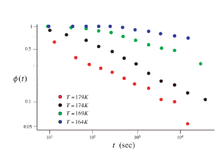
Figure 1: Experimental relaxation in MbCO icko

It is of interest to ask whether there is a model of hierarchically constrained dynamics as proposed in Ref. g4, which can account for the main features of Fig. 1. These are: a) At each temperature there is a region of power-law relaxation which crosses over at shorter times to something much slower. b) This crossover time increases as temperature decreases. c) The power law is the same at each temperature, but there is an increasing offset as the temperature is lowered.

In what follows, it will be shown that one of the models mentioned in Ref. g4, in fact gives behavior identical to what was observed in MbCO. For HCD, one recognizes that equilibrium distributions in configuration space are not relevant since the free energy barriers which determine relaxation are continuously changing in time as different degrees of freedom relax at different rates. Furthermore, in a strongly correlated system one expects that with any choice of coordinates, interactions will remain in the form of constraints and that these will be of importance over a range of time scales. The nature of constraints is that some degrees of freedom cannot relax until their motion is made possible by the relaxation of other degrees of freedom. These restrictions occur over a wide hierarchy of coordinates, from fast ones to slow ones. A complete discussion of this HCD approach is given in Ref. g4, .

To implement this picture, Palmer et al. g4 set up a hierarchy of levels $n=0,1,2,3,\ldots$. The degrees of freedom in level $n$ are represented by $N_{n}$ Ising pseudospins (two-level centers) each of which has two possible states. This was adapted from earlier work of Stein dls . Constraints enter via the requirement that each “spin” in level $n+1$ is free to change its state only if a condition on some number $\mu_{n}$ of spins in level $n$ is satisfied. Now, the $\mu_{n}$ spins have $2^{\mu_{n}}$ states. Let the required condition be that just one of these possible states is realized. If the average relaxation time in level $n$ is $\tau_{n}$, then on average, it will take a time $2^{\mu_{n}}\tau_{n}$ for a spin in level $n+1$ to change its state. Therefore

$$\tau_{n}=\tau_{0}\prod_{0}^{n-1}\exp(\mu_{i}\ln 2)=\tau_{0}\exp U_{n},$$ (3)

where

$$U_{n}=\sum_{0}^{n-1}\mu_{i}\ln 2.$$ (4)

The relaxation function is given as a sum of the correlation functions of all the degrees of freedom $S_{i}$:

$$\Phi(t)=(1/N)\sum_{i=1}^{N}\langle S_{i}(0)S_{i}(t)\rangle.$$ (5)

In a correlated system, the dynamics of the $S_{i}$ are not independent, so each of the correlation functions in Eq. (5) depends on the behavior of the other $S$’s. As described above, the HCD scheme of Palmer et al. g4 incorporates correlations. The $S_{i}$ are arranged in a hierarchy of levels $n$ with each level having its characteristic relaxation time $\tau_{n}$ given by Eq. (3). So Eq. (5) may be rewritten as a sum over the different levels from 0 to $\infty$:

$$\Phi(t)=\sum_{n=0}^{\infty}w_{n}\exp(-t/\tau_{n}),$$ (6)

where $w_{n}=N_{n}/N$ is the fraction of the total number of degrees of freedom which are in level $n$. finite

For a given model, $w_{n}$ and $\mu_{n}$ must be specified. As remarked in Ref. g4, , the simple choices $\mu_{n}=\mu_{0}/\ln 2$, a constant and $w_{n}=w_{n-1}/\lambda$ give power-law relaxation. Here, this situation is examined more fully.

The sum in Eq. (6) is rewritten as an integral using the above choices for $w$ and $\mu$:

$$\Phi(t)=w_{0}\int_{0}^{\infty}dn\lambda^{-n}\exp[(-t/\tau_{0})e^{-n\mu_{0}}],$$ (7)

where from normalization at $t=0$, $w_{0}=\ln\lambda$. This integral is evaluated exactly in terms of the incomplete gamma function

$$\gamma(\nu,u)=\int_{0}^{u}dx\,x^{\nu-1}e^{-x}.$$ (8)

The result is

$$\Phi(t)=\nu\left(\frac{\tau_{0}}{t}\right)^{\nu}\gamma(\nu,t/\tau_{0}),$$ (9)

where $\nu\equiv\ln\lambda/\mu_{0}$. For large values of its second argument, $\gamma(\nu,u)$ approaches the complete gamma function $\Gamma(\nu)$. Thus, at large times $\Phi(t)\propto t^{-\nu}$, as observed icko . For small $u$, $\gamma(\nu,u)\approx u^{\nu}/\nu-u^{\nu+1}/(\nu+1)+\ldots$, so that for short times, $\Phi(t)$ crosses over to a slower $1-{\rm const}(t/\tau_{0})$ dependence. Temperature dependence is introduced in the model through the temperature dependence of the fundamental relaxation time $\tau_{0}(T)$; its inverse corresponds to the rate constant $k_{r}(T)$ introduced in Ref. icko, . Thus the behavior of Eq. (9) is similar to the form

$$\Phi(t)=[1+k_{r}(T)\,t\,]^{-\nu}$$ (10)

which was used in Fig. 3 of Ref. icko, to fit the data.

The appearance of the experimental points at different temperatures, in particular that the data are parallel (the same power law for all $T$) at long times, suggests that a scaling function could describe the experimental results. A general form is

$$\Phi(t,T)\propto T^{\alpha}G[t/\tau_{0}(T)],$$ (11)

Therefore, by rescaling the time by a parameter $\tau_{0}(T)$ for each temperature the data for $\Phi(t,T)/T^{\alpha}$ would all fall on a single curve. The fact that the power law of the long time behavior is independent of $T$ implies that the exponent $\alpha=0$. If this rescaling is carried out, the temperature dependence of the characteristic rescaling time $\tau_{0}(T)$ may be determined. This rescaling for the data of Iben et al icko is shown in Fig. 2a.

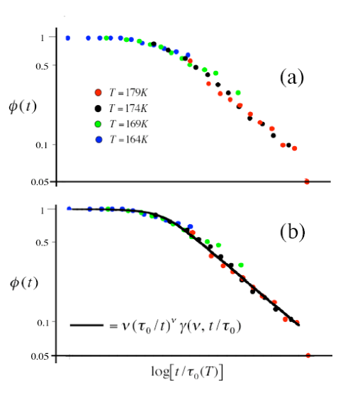
Figure 2: (a) Rescaled data of Iben et al. icko     (b) Comparison of theory and rescaled data

If in addition one has a theoretical expression which has a scaling form, such as Eq. (9), then by collapsing the data onto the theoretical curve, one obtains the numerical values of $\tau_{0}(T)$. This is carried out for the hierarchical model of Eq. (9) in Fig. 2b. The value of $\nu$ in Eq. (9) is adjusted to agree with the common large $t$ slope as seen in Fig. 2a. The black curve in Fig. 2b is Eq. (9) with $\nu$ set equal to 0.28. The values of $\tau_{0}$ for each of the four temperatures are plotted in Fig. 3, where the solid curve is a fit using the expression

$$1/\tau_{0}(T)=k_{0}\exp[-(T_{0}/T)^{2}]$$ (12)

The result is $k_{0}=1.5\times 10^{16}\;{5\rm s}^{-1},\;T_{0}=1105$ K.cf

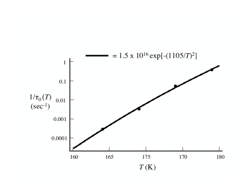
Figure 3: Fundamental relaxation rate

With only four points, a number of different functional forms might seem equally good. In particular, an Arrhenius form works almost as well, but has an unacceptably large pre-exponential factor. pnas The form chosen has been suggested by several authors icko ; bass ; it can describe diffusion in a random potential of a form which mimics the potential surface of a protein.

As discussed in Ref. icko, , the observed relaxation process most likely involves substates having different conformational molecular structures as well as different angles of the CO ligand with respect to the heme normal. With this in mind, contact may be made between the parameters of the above model and the actual experiment. Recall that $\mu_{0}$ measures the number of “spins” in a given level which must arrive at a certain configuration before a typical spin in the next level becomes unfrozen and can relax. The physical picture of constrained movement of atoms which underlies the model and its application to MbCO then implies that this number should be around 3 to 5 or so. The number $\lambda$ measures the geometric reduction of the fraction of spins which belong to level $n$ as $n$ increases through slower and slower levels. $\Phi(t)$ has only a logarithmic dependence on $\lambda$ so it is reasonable to take $\ln\lambda$ to be of order unity. This gives $\nu=\ln\lambda/\mu_{0}\lesssim 1$. The fit value is $\nu=0.28$, i.e. slightly less than four spins, on average, combine to unfreeze the degrees of freedom at the next level. This seems quite reasonable.

Eq. (10), taken from Eq. (1) of Ref. icko, is consistent with the present Eq. (9) in that they agree in the limits of small and large $t/\tau_{0}$. Therefore the fit by Iben et al. icko using Eq. (10) is also satisfactory. However, there is no physical motivation for that form whereas in the present work the observed non-exponential relaxation in MbCO is derived from a microscopic model which incorporates strong-correlation constraints on the relaxation of the molecule in a definite way.

What conclusions can be drawn from the present analysis? The scenario that the model describes is one in which the primary relaxation event represents the rate $1/\tau_{0}(T)$ at which a typical enthalpy barrier is overcome. Since no further $T$-dependence is introduced, the conclusion is that all subsequent relaxation events are “slaved”pnas to the primary one and that they represent entropic conformational changes of the molecule.

A Los Alamos group has independently been analyzing the relaxation processes in MbCO. pnas ; lanl Remarkably, they have reached conclusions which are consistent with the present hierarchical model for the relaxation of the CO vibration frequency. Namely, they argue that the temperature dependence of the relaxation is governed by an activation enthalpy for which the solvent is responsible. This determines the rate of the fastest relaxation process - $1/\tau_{0}(T)$ in the hierarchical model. Subsequent relaxations involve degrees of freedom of the protein and the hydration shell and are governed by entropy barriers; they have the same temperature dependence as the solvent fluctuation rate and are slower. This description is precisely the same as that of the hierarchical model presented here. The physically motivated scenario of the successful hierarchical approach lends support to the identification of the physical relaxation processes described in Ref. 12.

The analysis presented here can be generalized to more complicated situations. For example, the hierarchical rules could be modified to include simultaneous parallel relaxation (“unslaved”) processes as in the ligand rebinding referred to earlier, internal enthalpic barriers, reverse constraints, and intra-level correlations. While other forms than Eq. (9) might fit the MbCO data, within the hierarchical scenario the fact that the long time behavior is a scalable power law practically forces the simple rules which were used to obtain Eq. (9). The success of this approach suggests that a similar picture and analysis can be relevant for other dynamical processes in biological molecules. If so, insight can be obtained about the physical processes which determine the relaxation phenomena.

The author wishes to acknowledge helpful and often critical discussions with R. Austin, S. Doniach, P. Fenimore, H. Frauenfelder, B. McMahon, B. Shklovskii, D. Stein. A portion of this work was carried out during the author’s participation in activities of the Institute for Complex Adaptive Matter (ICAM). The hospitality of the Aspen Center for Physics, where the research was begun and completed, is gratefully acknowledged.

References

- (1) V.I. Goldanskii, Yu.F. Krupyanskii and V.N. Flerov, Dokl. Akad. Nauk SSSR 272, 978 (1983).
- (2) D.L. Stein, Proc. Natl. Acad. Sci. USA 82, 3670 (1985).
- (3) I.E.T. Iben, et al.., Phys. Rev. Lett. 62, 1916 (1989).
- (4) Y. Shibata, A. Kurita, and T. Kushida, Biochemistry 38, 1789-1801 (1999).
- (5) H. Vogel, Phys. Z. 22, 645 (1921); G.S. Fulcher, J. Am. Ceram. Soc. 8, 339 (1925).
- (6) R.G. Palmer, D.L. Stein, E. Abrahams, and P.W. Anderson, Phys. Rev. Lett. 53, 958 (1984).
- (7) R.H. Austin, K.W. Beeson, L. Eisenstein, and H. Frauenfelder, Biochemistry, 14, 5355 (1975); Noam Agmon and J.J. Hopfield, J. Chem. Phys. 79, 2042 (1983).
- (8) One may ask whether taking an infinite sum in Eq. (6) would be appropriate for a finite system. It can be checked that for the analysis which follows for MbCO, taking a finite sum over only 3 levels, say, gives less than a 10% correction to the relaxation function at long times.
- (9) H. Bässler, Phys. Rev. Lett. 58, 767 (1987); M. Grünewald, et al.., Philos. Mag. B 49, 341 (1984); R. Zwanzig, Proc Natl. Acad. Sci. USA. 85, 2029 (1988)¿
- (10) These numbers are of course rather close to the ones determined in Ref. 1: K
- (11) P.W. Fenimore, H. Frauenfelder, B.H. McMahon, and F.G. Parak, Proc. Natl. Acad. Sci. USA 99, 16047 (2002).
- (12) P.W. Fenimore, H. Frauenfelder, B.H. McMahon, and R.D. Young, Proc. Natl. Acad. Sci. USA 101, 14408 (2004).