Supersymmetric Free-Damped Oscillators: Adaptive Observer Estimation of the Riccati Parameter

Abstract

A supersymmetric class of free damped oscillators with three parameters has been obtained in 1998 by Rosu and Reyes through the factorization of the Newton equation. The supplementary parameter is the integration constant of the general Riccati solution. The estimation of the latter parameter is performed here by employing the recent adaptive observer scheme of Besançon et al., but applied in a nonstandard form in which a time-varying quantity containing the unknown Riccati parameter is estimated first. Results of computer simulations are presented to illustrate the good feasibility of this approach for a case in which the estimation is not easily accomplished by other means.

Key Words: three-parameter free-damped oscillator; adaptive observer; Riccati parameter.

PACS numbers: 87.10.+e, 02.30.Yy.

Int. J. Theor. Phys. Vol. 45, No. 11, Nov. 2006, 2109-2117.
Rec. Dec. 28, 2005; accept. Feb. 14, 2006; online Sept. 22, 2006. physics/0411019v2, papptp2.tex

1 Three-parameter Free-damped Modes

In 1998, Rosu and Reyes [1] introduced classical three-parameter free damped oscillators by means of the nonrelativistic supersymmetry (factorization) technique. They showed that in this approach the usual two-parameter free damped oscillator equation (the dots are for time derivatives)

$$y^{{}^{\prime\prime}}+2\beta y^{{}^{\prime}}+\omega_{0}^{2}y=0$$

is generalized to a damped oscillator equation of the form

$$\tilde{y}^{{}^{\prime\prime}}+2\beta\tilde{y}^{{}^{\prime}}+\omega^{2}(t;\gamma)\tilde{y}=0~{},\,\,{\rm where}\,\,\quad\omega^{2}(t;\gamma)=\Big{[}\omega_{0}^{2}-\frac{2\gamma^{2}}{(\gamma t+1)^{2}}\Big{]}~{},$$ (1)

possessing damping solutions with singularities that we call here $\gamma$ modes, see below. The new damping solutions depend on an additional parameter $\gamma$ given by the general Riccati solution associated to the original two-parameter damped equation. This $\gamma$ parameter introduces a new time scale in the damping phenomena that is related to the time at which the singularities occur.

For the three types of free damping, the $\gamma$ modes are the following:

(i) Underdamping: $\beta^{2}<\omega_{0}^{2}$, $\omega_{u}=\sqrt{\omega_{0}^{2}-\beta^{2}}$

$$\tilde{y}_{u}=-\tilde{A}_{u}e^{-\beta t}\Big{[}\omega_{u}\sin(\omega_{u}t+\phi)+\frac{\gamma}{\gamma t+1}\cos(\omega_{u}t+\phi)\Big{]}~{}.$$ (2)

(ii) Overdamping, $\beta^{2}>\omega_{0}^{2}$, $\omega_{o}=\sqrt{\beta^{2}-\omega_{0}^{2}}$,

$$\tilde{y}_{0}=-\tilde{A}_{o}e^{-\beta t}\Big{[}\omega_{o}\sinh(\omega_{o}t+\phi)-\frac{\gamma}{\gamma t+1}\cosh(\omega_{o}t+\phi)\Big{]}~{}.$$ (3)

(iii) Critical damping, $\beta^{2}=\omega_{0}^{2}$.

$$\tilde{y}_{c}=e^{-\beta t}\Big{[}\frac{-A_{c}\gamma}{\gamma t+1}+\frac{D_{c}}{\gamma^{2}}(\gamma t+1)^{2}\Big{]}~{}.$$ (4)

Damped motion of this type could be quite common in nature, although if the value of $\gamma$ is very small it is difficult to distinguish it from the usual two-parameter free damping. In such cases it is still possible to estimate $\gamma$ through some powerful estimation methods. The problem of parameter estimation in dynamical systems has motivated extensive studies of the adaptive observer designs for linear and nonlinear systems during the last decade. Among the single output adaptive schemes that can be directly applied to our case we cite those of Marino,[2] Marino and Tomei,[3] and Besançon.[4] It is the purpose of this paper to show that very good estimates for $\gamma$ can be obtained by applying the latter scheme. The main reason to use the Besançon scheme is its simplicity with respect to the scheme of Marino that requires solving more differential equations in real time in order to obtain the corresponding velocity to recover the unknown value of the parameter(s). In the next section, Eq. (1) is written as a system of two first-order differential equations in the affine form which is required in order to apply Besançon’s adaptive observer scheme. This is detailed in Section 3 where we also give some pedestrian definitions of the technical concepts involved in the adaptive estimation algorithms. A small conclusion section ends up the paper.

2 Equivalent System of First Order Differential Equations

Denoting $X_{1}=\tilde{y}$ and $X_{2}=\dot{\tilde{y}}$, Eq. (1) can be rewritten as

$$\dot{X_{1}} = X_{2}$$ (5)

$$\dot{X_{2}} = -2\beta X_{2}+\left(\frac{2\gamma^{2}}{(\gamma t+1)^{2}}-\omega_{0}^{2}\right)X_{1}~{}.$$ (6)

We will consider $X_{1}$ as the naturally measured state (the most easy to measure). Therefore, it seems logical to take $X_{1}$ as the output of the system, that is $y=CX$, where $C=[1\ 0]$ and $X$ is state vector. In addition, we consider that $\beta$ is available in some way and only $\gamma$ stands as an unknown parameter. Thus, the complete monitoring of the system means the on-line estimation of $X_{2}$ and the on-line identification of the $\gamma$ value. The available methods for parameter identification need that the unknown parameters are in affine form, i.e.

$$\dot{X_{1}} = X_{2}$$ (7)

$$\dot{X_{2}} = -2\beta X_{2}+\alpha X_{1}~{},$$ (8)

where $\alpha$ is the unknown constant parameter. It is clear that $\gamma$ is not an affine parameter but we can try to estimate the time-dependent quantity

$$\alpha(t)=\left(\frac{2\gamma^{2}}{(\gamma t+1)^{2}}-\omega_{0}^{2}\right)~{},$$ (9)

because it appears in the affine form. Notice that, even though $\alpha$ is not a constant, its evolution is significant only close to the origin, that is, as time increases $\alpha$ turns rapidly into a constant parameter.

3 Design of the Adaptive Observer

It is well known that only in very special occasions one can have a sensor on every state variable, and some form of reconstruction from the available measurement output data is needed, in many cases. In general, an observer is an algorithm that reconstructs the unmeasurable states of a system from the measurable output. The so-called high gain techniques proved to be very efficient for state estimation, leading to the well-known concept of high gain observer [5]. The gain is the amount of increase in error in the observer’s structure. This amount is directly related to the velocity with which the observer recovers the unknown signal. The high-gain observer is an algorithm in which the amount of increase in error is constant and usually of high values in order to achieve a fast recover of the unmeasurable states. However, when a system depends on some unknown parameters, the design of the observer has to be modified in such a way that the state variables and parameters could be estimated. This leads to the so called adaptive observers, i.e., observers that can change in order to work better or provide more fit for a particular purpose.

Here, we present an interesting application of the recent scheme of Besançon and collaborators,[4] for unknown parameters that appear linearly in the dynamical system to the interesting case of state and parameter estimation of the three-parameter free-damped oscillator. In this particular case, the unknown parameter appears in a nonlinear manner and in order to avoid this difficulty we group together a set of parameters which leads to a time-dependent parameter. The block scheme of the adaptive observer for this case is presented in Fig. (1).

The main assumptions on the considered class of systems are that if all parameters were known, some high-gain observer could be designed in a classical way, and that the systems are “sufficiently excited” in a sense which is close to the usually required assumption on adaptive systems (the signals must be rich enough so that the unknown parameters can indeed be identified).

We write the $\gamma$ free damping motion system given by Eqs. (7)-(8) in Besançon’s form:

$$\text{$\ \ \ \digamma$ =}\left\{\begin{array}[]{@{}l@{\quad}l@{}}\dot{X}=AX+\varphi(X)+\Psi(X){\theta}\\ y=CX\end{array}\ \right.$$

where:

$A$ - Brunovsky-type matrix, i.e., of the form $A=\delta_{i,j+1}$, where $\delta_{ij}$ is the Kronecker symbol

$X^{n}\in\mathbb{R}$ - $n$-component real vector

$y$ - measured output

$\Psi(t)\in\mathbb{R}^{n\times p}$ - the vector of known functions ($p$ = the number of unknown parameters)

$\theta\in\mathbb{R}^{p}$ - vector of unknown parameters (i.e., a vector belonging to some known compact set that should be estimated through the measurements of the output $y$).

For the $\gamma$ system, we have: $n=2$, $p=1$ and $\theta=\alpha$.

Therefore the entries of the matrix $A$ are $a_{11}=0$, $a_{12}=1$, $a_{21}=0$ and $a_{2,2}=0$, the entries of the vector $\Psi$ are $\psi_{11}=0$ and $\psi_{21}=X_{1}$, whereas the entries of the vector $\varphi$ are $\varphi_{11}=0$ and $\varphi_{21}=-2\beta X_{2}$.

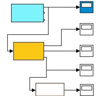
Figure 1: Schematic representation of the adaptive observer, where the output of the system is the input of the adaptive observer and the outputs of the latter are the rebuilt states and the parameter $\alpha$ from which it is possible to rebuild $\gamma$.

We consider now the following dynamical system

$$\text{$\ \ \ \hat{\digamma}$=}\left\{\begin{array}[]{@{}l@{\quad}l@{}}\dot{\hat{X}}=A\hat{X}+\varphi(\sigma(\hat{X}))+\Psi(\sigma({\hat{X}}))\sigma({\theta})+\Lambda^{-1}\left[\rho K+\Gamma\Gamma^{T}C^{T}\right]\left(y-C\hat{X}\right)\\ \dot{\hat{\theta}}=\left[\rho^{n}\Gamma^{T}C^{T}\right]\left(y-C\hat{X}\right)\\ \dot{\hat{\Gamma}}=\rho\left(A-KC\right)\Gamma+\rho\Psi(\sigma(\hat{X}))~{},\end{array}\ \right.$$

where $\Gamma\in\mathbb{R}^{n\times p}$, $K$ is some vector for which $A-KC$ is a stable matrix, $\Lambda={\rm diag}[1,\rho^{-1},\ldots,\rho^{-(n-1)}]$, $\rho\in\mathbb{R}_{+}$ being a constant to be chosen, and $\sigma$ is a so-called saturation function. The saturation function is a map whose image is bounded by the chosen upper and lower limits, $B$ and $b$, respectively [6]. This avoids the over and/or under estimation, keeping the possible values within the set of the physically reliable values, and consequently increasing the chance of the quick convergence to the true values. Thus, the latter is the following map

$$\sigma(s)=\left\{\begin{array}[]{@{}l@{\quad}l@{}}B$\quad$s>B\\ s$\quad$b\leq s\leq B\\ b$\quad$s<b~{}.\end{array}\ \right.$$

$\hat{\digamma}$ has been proven by Besançon to be a global exponential adaptive observer for the system $\digamma$. That means that for any initial conditions $X(t_{0})$, $\hat{X}(t_{0})$, $\hat{\theta}(t_{0})$ and $\forall\theta\in\mathbb{R}^{p}$, the errors $\hat{X}(t)-X(t)$ and $\hat{\theta}(t)-\theta(t)$ tend to zero exponentially fast when $t\rightarrow\infty$. Consequently, for the free damping motion system, the matrix $A-KC$ has the eigenvalues

$$\lambda_{1,2}=-1/2\,k_{{1}}\pm 1/2\,\sqrt{{k_{{1}}}^{2}-4\,k_{{2}}}$$ (10)

Selecting $k_{2}=\left(\frac{k_{1}}{2}\right)^{2}$, we get the eigenvalues $\lambda_{1}=\lambda_{2}=-k_{1}/2$, and choosing any $k_{1}>0$ we make $A-KC$ a stable matrix. Thus, the explicit non matrix form of the observer given by $\hat{\digamma}$ is the following

$$\dot{\hat{X}}_{1} = \hat{X}_{2}+\left(\rho k_{1}+{\Gamma_{1}}^{2}\right)(X_{1}-\hat{X}_{1})$$

$$\dot{\hat{X}}_{2} = -2\beta\sigma(\hat{X}_{2})+\sigma(\hat{X}_{1})\sigma(\hat{\theta})+\rho\left(\frac{\rho{K_{1}}^{2}}{4}+\Gamma_{1}\Gamma_{2}\right)(X_{1}-\hat{X}_{1})$$

$$\dot{\hat{\theta}} = \rho^{2}\Gamma_{1}(X_{1}-\hat{X}_{1})$$

$$\dot{\Gamma}_{1} = \rho(-k_{1}\Gamma_{1}+\Gamma_{2})$$

$$\dot{\Gamma}_{2} = -\frac{1}{4}\rho{k_{1}}^{2}\Gamma_{1}+\rho\sigma(\hat{X}_{1}))~{}.$$

To recover now the value of the parameter $\gamma$ from the estimated value of $\alpha$, we solve for $\gamma$ the equation $2[\gamma/(\gamma t+1)]^{2}-\omega_{0}^{2}=\alpha$, giving

$$\gamma={\frac{-t(\alpha\,t+{\beta}^{2})-\sqrt{2\,\alpha+2\,{\beta}^{2}}}{t^{2}(\alpha+{\beta}^{2})-2}}~{}.$$ (11)

We still can hope that the value of $\gamma$ can be estimated with sufficiently good accuracy until the blow-up time $t_{d}=\sqrt{2}/\left(\alpha+\beta^{2}\right)^{\frac{1}{2}}$ and indeed this is what we have found for the $\gamma$ modes.

In the computer simulations that we performed for illustrating purpose we took always $\rho=100$ for the constant parameter defining the diagonal matrix $\Lambda$. Figures (2) - (5) show the results of numerical simulations for an underdamped case with the following parameters: $\beta=0.04$, $\gamma=0.15$, $k=1.00$, $\omega_{0}=1.00$. In figure (6), we present numerical simulations for the Riccati parameter $\gamma$ for the overdamped case with $\beta=1.0$ and $\omega_{0}=0.2$ in the plot (a) and the critical case with $\beta=\omega_{0}=0.1$ in the plot (b). Figure 5a shows the initial stages of the process of convergence displaying big oscillations. After this, one can always notice the convergence to the true value once the estimate enters the neighborhood of the true value determined by the exponential criterium of convergence to the neighborhood, where small oscillations around the true value are quite natural. The numerical simulations have been performed with the relative values of the parameters chosen to illustrate the three classes of damping, but otherwise there are no restrictions on their values.

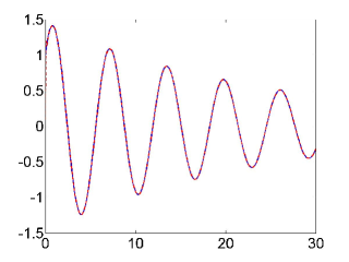
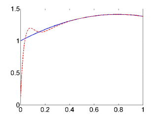
Figure 2: Numerical simulations for the state $X_{1}$ in the underdamping case. In (a) the solid line represents the time evolution of the true state and the dotted line gives the evolution of its estimate. The plot (b) is a detail of the figure (a) to appreciate the variation of $\hat{X_{1}}$ in the beginning.

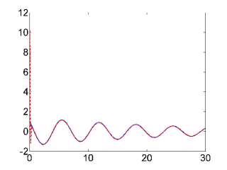
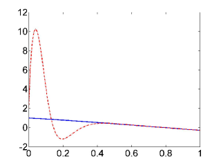
Figure 3: Numerical simulation for the state $X_{2}$ in the underdamping case. In (a) the solid line represents the time evolution of the true state and the dotted line gives the evolution of its estimate. Plot (b) is a detail of (a) to see better the variation of $\hat{X_{2}}$ in the beginning.

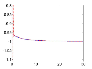
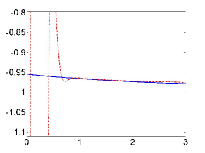
Figure 4: Numerical simulation for $\alpha$ in the underdamping case. The solid line represents the true value of $\alpha$ and the dotted line gives the estimate. Plot (b) is a detail of (a) to see better the variation of the estimated $\alpha$ in the beginning.

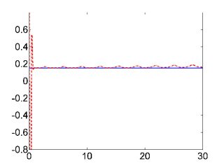
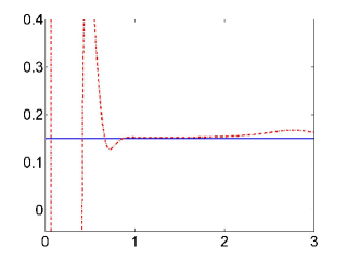
Figure 5: Numerical simulation for the parameter $\gamma$ in the underdamping case. The true value of $\gamma$ is given by the solid line whereas the dotted line gives the estimate. Plot (b) gives the details of (a) near the origin to better see the variation of the estimate of $\gamma$.

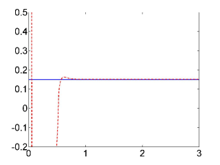
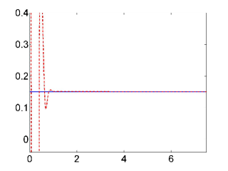
Figure 6: Numerical simulations for the parameter $\gamma$ in the overdamped case [plot (a)], and in the critical case [plot (b)]. The solid line gives the true value of $\gamma$ and the dotted line gives its estimate.

4 Conclusion

The adaptive observer scheme of Besançon et al is an effective procedure to rebuild the Riccati parameter of the class of damping modes of Rosu and Reyes. Despite the fact that in the estimation algorithm we used an associated time-varying quantity for which the exponential convergence is not guaranteed, we obtain excellent results for the estimates of the unknown constant Riccati parameter. As it can be seen from this work, the application of Besançon’s adaptive scheme is not necessarily restricted to the estimation of constant parameters but one can go with it to some time-varying cases. In addition, the scheme provides very good estimates for the unknown states of this class of oscillators for each of the three possible cases. Moreover, the rapid identification of the additional parameter $\gamma$ of the chirped damped oscillators by this method opens a way to the experimental study of these oscillators.

References

- [1] H.C. Rosu and M.A. Reyes, Riccati parameter modes from Newtonian free damping motion by supersymmetry, Phys. Rev. E 57, 4850 (1998); H.C. Rosu and P.B. Espinoza, Ermakov-Lewis angles for one-parameter susy families of Newtonian free damping modes, Phys. Rev. E 63, 037603 (2001).
- [2] R. Marino, Adaptive observer for single output nonlinear systems, IEEE Trans. Autom. Control 35, 1054 (1990).
- [3] R. Marino and P. Tomei, Adaptive observer with arbitrary exponential rate of convergence for nonlinear systems, IEEE Trans. Autom. Control 40, 1300 (1995).
- [4] G. Besançon, O. Zhang, and H. Hammouri, High gain observer based state and parameter estimation in nonlinear systems, paper 204 in the 6th Int. Fed. Aut. Ctrl. Symposium, Stuttgart Symposium on Nonlinear Control Systems, (2004), available at http://www.nolcos2004.uni-stuttgart.de.
- [5] J.P. Gauthier, H. Hammouri, and S. Othman, A simple observer for nonliner systems: applications to bioreactors, IEEE Trans. Autom. Control 37, 875 (1992).
- [6] H.K. Khalil, Nonlinear Systems, (Prentice-Hall, Inc., 1992).