Exact semi-relativistic model for ionization of atomic hydrogen by electron impact

Abstract

We present a semi-relativistic model for the description of the ionization process of atomic hydrogen by electron impact in the first Born approximation by using the Darwin wave function to describe the bound state of atomic hydrogen and the Sommerfeld-Maue wave function to describe the ejected electron. This model, accurate to first order in $Z/c$ in the relativistic correction, shows that, even at low kinetic energies of the incident electron, spin effects are small but not negligible. These effects become noticeable with increasing incident electron energies. All analytical calculations are exact and our semi-relativistic results are compared with the results obtained in the non relativistic Coulomb Born Approximation both for the coplanar asymmetric and the binary coplanar geometries.

I Introduction

Relativistic $(e,2e)$ processes have been reviewed both from the experimental and theoretical point of view [1]. As one deals with atomic hydrogen, the value of the parameter $Z\alpha$ is very lower than one, where $Z$ is the atomic charge number and $\alpha$ is the fine structure constant. Therefore, it is convenient and sufficient to use approximate wave functions of a mathematically simpler structure than the exact analytical wave functions needed to describe relativistic $(e,2e)$ processes. A numerical approach to an exact description of the relativistic ionization of atomic hydrogen by electron impact could be carried out but we will focus instead on an alternative approach that will give nearly the same results as the exact description if the condition $Z\alpha\ll 1$ is satisfied. In $(e,2e)$ processes, relativistic effects are important and all electrons (the incident, scattered and ejected) can have very high velocities. One has to consider many interactions (to name some, retardation interaction, magnetic interaction and spin-dependent interaction). For atomic hydrogen, many experimental and theoretical contributions have been made [2-3]. Some were successful but the theoretical situation for all set-ups and kinematics is far from resolved, at least analytically. Many calculations have resorted to various approximations. For example, plane wave models [4-7] are successful in the coplanar binary geometries [4] and for fast scattered and ejected electrons. The first Born approximation (FBA) has been used to describe asymmetric geometries at non relativistic energies [8-9]. In this approximation, the incident and scattered electrons are described by plane waves whereas the ejected electron is treated as a Coulomb wave. Many authors extended this approximation to the relativistic domain. Das et al [10-11] employed a semi-relativistic Sommerfeld-Maue wave functions to describe the ejected electron. Jakubaßa-Amundsen evaluated the first-order transition matrix element $S_{fi}$ using semi-relativistic Coulomb wave functions times a free spinor i.e neglecting the relativistic contraction of the bound state and approximating the continuum Coulomb state by a relativistic Coulomb wave times a free spinor. This model did well in predicting integrated cross-sections [12] but yielded a value for the absolute triple differential cross section (TDCS) too large. For the Coulomb approximation, Jakubaßa-Amundsen argued that one could not neglect the Coulomb potential in the treatment of inner-shell ionization of high-$Z$ atoms. Agreement with experiment was encouraging for intermediate values of $Z$. The merits and shortcomings of this theory have been analyzed in [14]. Thereafter, a fully relativistic version was produced [15] which showed that the original physical insight was essentially correct.

In this contribution, we present a theoretical semi-relativistic model, the semi-relativistic Coulomb Born Approximation (SRCBA) in a closed and exact form for the description of the ionization of atomic hydrogen by electron impact that is valid for all geometries. Indeed, in the non relativistic Coulomb Born Approximation (NRCBA), a well known integral occurs [16] and is usually denoted by $I(\lambda)$. In this article, we show that the main contribution to the unpolarized triple differential cross section (TDCS) in the SRCBA corresponding to the ionization of atomic hydrogen in its ground state by electron impact comes from this term added to relativistic corrections valid to first order in $Z/c$. These relativistic corrections contain a new integral we have denoted $J(\lambda)$ and in the Appendix, we give the formal derivation of this integral. To our knowledge, it is the first time that such an integral is written down analytically. Needless to say that all numerical appropriate tests to check the validity of the analytical result we have found have been carried out with a very good degree of accuracy. It turns out that spin effects can be accounted for even at low kinetic energies of the incident electron in the case of the Ehrhardt coplanar asymmetric geometry [17] where, for a given kinetic energy $T_{i}$ of the fast incident electron, a fast (”scattered ”) electron of kinetic energy $T_{f}$ is detected in coincidence with a slow (”ejected”) electron of kinetic energy $T_{B}$. These spin effects as well as the relativistic effects become noticeable with increasing incident electron kinetic energy.

The organization of this paper is as follows : in section II, we present the semi relativistic formalism of $(e,2e)$ reaction and give a detailed account of the various terms that contribute to the unpolarized TDCS, in section III, we discuss the results we have obtained and we end by a brief conclusion in section IV. The formal derivation of the integral $J(\lambda)$ is given in the Appendix. Throughout this work, atomic units ($a.u$) are used $(\hbar=m_{e}=e=1)$ where $m_{e}$ is the electron rest mass.

II The unpolarized triple differential cross section

In this section, we calculate the exact analytical expression of the semi relativistic unpolarized TDCS in the SRCBA corresponding to the ionization of atomic hydrogen by electron impact. The transition matrix element for the direct channel (exchange effects are neglected) is given by

$$S_{fi} = -i\int dt<\psi_{p_{f}}(x_{1})\phi_{f}(x_{2})\mid V_{d}\mid\psi_{p_{i}}(x_{1})\phi_{i}(x_{2})>$$ (1)

$$= -i\int_{-\infty}^{+\infty}dt\int d\mathbf{r}_{1}\overline{\psi}_{p_{f}}(t,\mathbf{r}_{1})\gamma_{(1)}^{0}\psi_{p_{i}}(t,\mathbf{r}_{1})$$

$$\quad\quad\times<\phi_{f}(x_{2})\mid V_{d}\mid\phi_{i}(x_{2})>$$

In Eq. (1), $V_{d}$ is the direct interaction potential :

$$V_{d}=\frac{1}{r_{12}}-\frac{1}{r_{1}}$$ (2)

$\mathbf{r}_{1}$ are the coordinates of the incident and scattered electron, $\mathbf{r}_{2}$ are the atomic electron coordinates, $r_{12}=$ $\mid\mathbf{r}_{1}-\mathbf{r}_{2}\mid$ and $r_{1}=\mid\mathbf{r}_{1}\mid$. The wave function $\psi_{p_{i}}(x_{1})=\psi_{p}(t,\mathbf{r}_{1})=u(p,s)\exp(-ip.x)/\sqrt{2EV\text{ }}$ is the electron wave function described by a free Dirac spinor normalized to the volume $V$ and $\phi_{i,f}(x_{2})=\phi_{i,f}(t,\mathbf{r}_{2})$ are the semi relativistic wave functions of the hydrogen atom where the index $i$ stands for the initial state, namely the ground state and the index $f$ stands for the final state. The quantity $p.x=p_{\mu}x^{\mu}$ is the Lorentz scalar product. The semi relativistic wave function of the hydrogen atom used is the Darwin wave function for bound states [18]

$$\phi_{i}(t,\mathbf{r}_{2})=\exp(-i\varepsilon_{b}t)\varphi^{(\pm)}(\mathbf{r}_{2})$$ (3)

where

$$\varphi^{(\pm)}(\mathbf{r}_{2})=(\mathsf{1}_{4}-\frac{i}{2c}\mathbf{\alpha.\nabla}_{(2)})u^{(\pm)}\varphi_{0}(\mathbf{r}_{2})$$ (4)

is a quasi relativistic bound state wave function accurate to first order in $Z/c$ in the relativistic corrections (and normalized to the same order) with $\varphi_{0}$ being the non relativistic bound state hydrogenic function. The spinors $u^{(\pm)}$ are such that $u^{(+)}=(1,0,0,0)^{T}$ and $u^{(-)}=(0,1,0,0)^{T}$ and represent the basic four-component spinors for a particle at rest with spin-up and spin-down, respectively. For the spin up, we have

$$\varphi^{(+)}(\mathbf{r}_{2}) = N_{D}\left(\begin{array}[]{c}1\\ 0\\ \frac{i}{2c}\cos\theta_{2}\\ \frac{i}{2c}\sin(\theta_{2})\exp(i\phi_{2})\end{array}\right)\frac{1}{\sqrt{\pi}}e^{-r_{2}}$$ (9)

and for the spin down, we have

$$\varphi^{(-)}(\mathbf{r}_{2}) = N_{D}\left(\begin{array}[]{c}0\\ 1\\ \frac{i}{2c}\sin(\theta_{2})\exp(-i\phi_{2})\\ -\frac{i}{2c}\cos(\theta_{2})\end{array}\right)\frac{1}{\sqrt{\pi}}e^{-r_{2}}$$ (14)

where

$$N_{D}=2c/\sqrt{4c^{2}+1}$$ (15)

is a normalization constant lower but very close to one. The wave function $\phi_{f}(t,\mathbf{r}_{2})$ in Eq. (1) is the Sommerfeld-Maue wave function for continuum states [18] also accurate to the order $Z/c$ in the relativistic corrections. We have $\phi_{f}(t,\mathbf{r}_{2})=\exp(-iE_{b}t)\psi_{p_{f}}^{(-)}(\mathbf{r}_{2})$ and

$$\psi_{p_{f}}^{(-)}(\mathbf{r}_{2})=\exp(\pi\eta_{B}/2)\Gamma(1+i\eta_{B})\exp(i\mathbf{p}_{B}.\mathbf{r}_{2})$$ (16)

$$\times \big{\{}\mathsf{1}_{4}-\frac{ic}{2E_{B}}\mathbf{\alpha}.\mathbf{\nabla}_{(2)}\big{\}}\,_{1}F_{1}(-i\eta_{B},1,-i(p_{B}r_{2}+\mathbf{p}_{B}.\mathbf{r}_{2}))$$

$$\times \frac{u(p_{B},s_{B})}{\sqrt{2E_{B}V}}$$

normalized to the volume $V$. The Sommerfeld parameter is given by

$$\eta_{B}=\frac{E_{B}}{c^{2}p_{B}}$$ (17)

In Eqs. (3) and (8), $\mathbf{\alpha}$ is related to the $\mathbf{\gamma}$ Dirac matrices [19] and in the standard representation reads

$$\mathbf{\alpha}=\left(\begin{array}[]{ll}0&\mathbf{\sigma}\\ \mathbf{\sigma}&0\end{array}\right)$$ (18)

with $\mathbf{\sigma=}(\sigma_{x},\sigma_{y},\sigma_{z})$ and the matrices $\sigma_{x},\sigma_{y},\ \sigma_{z}$ are the usual Pauli matrices. The matrix differential operator $\mathbf{\mathbf{\alpha}.\mathbf{\nabla}}$ is given by

$$\mathbf{\mathbf{\alpha}.\mathbf{\nabla}=}\left(\begin{array}[]{llll}0&0&\partial_{z}&\partial_{x}-i\partial_{y}\\ 0&0&\partial_{x}+i\partial_{y}&-\partial_{z}\\ \partial_{z}&\partial_{x}-i\partial_{y}&0&0\\ \partial_{x}+i\partial_{y}&-\partial_{z}&0&0\end{array}\right)$$ (19)

We give the final compact form of the Sommerfed-Maue wave function

$$\psi_{p_{f}}^{(-)}(\mathbf{r}_{2})=\exp(\pi\eta_{B}/2)\Gamma(1+i\eta_{B})\exp(i\mathbf{p}_{B}.\mathbf{r}_{2})\Big{\{}\,_{1}F_{1}(-i\eta_{B},1,-i(p_{B}r_{2}+\mathbf{p}_{B}.\mathbf{r}_{2}) +\frac{i}{2cp_{B}}(\mathbf{\alpha.p}_{B}+p_{B}\mathbf{\alpha.}\widehat{\mathbf{r}}_{2})$$

$$\times_{1}F_{1}(-i\eta_{B}+1,2,-i(p_{B}r_{2}+\mathbf{p}_{B}.\mathbf{r}_{2}))\Big{\}}\frac{u(p_{B},s_{B})}{\sqrt{2E_{B}V}}$$ (20)

In Eq. (12), the operator $\mathbf{\alpha.p}_{B}$ acts on the free spinor $u(p_{B},s_{B})$ and the operator $\mathbf{\alpha.}\widehat{\mathbf{r}}_{2}$ acts on the spinor part of the Darwin function. The direct transition matrix element in Eq. (1) becomes

$$S_{fi} = -i\int d\mathbf{r}\frac{\overline{u}(p_{f},s_{f})}{\sqrt{2E_{f}V}}\gamma_{(1)}^{0}\frac{\overline{u}(p_{B},s_{B})}{\sqrt{2E_{B}V}}\gamma_{(2)}^{0}\Big{\{}\,_{1}F_{1}(i\eta_{B},1,i(p_{B}r+\mathbf{p}_{B}.\mathbf{r})\mathsf{1}_{4}-\frac{i}{2cp_{B}}(\mathbf{\alpha.p}_{B}+p_{B}\mathbf{\alpha.}\widehat{\mathbf{r}})$$ (21)

$$\times {}_{1}F_{1}(i\eta_{B}+1,2,i(p_{B}r+\mathbf{p}_{B}.\mathbf{r}))\Big{\}}\varphi^{(\pm)}(\mathbf{r})\exp(-i\mathbf{p}_{B}.\mathbf{r})[\exp(i\mathbf{\Delta.r})-1]$$

$$\times \frac{8\pi^{2}}{\Delta^{2}}\delta(E_{f}+E_{B}-E_{i}-\varepsilon_{b})\frac{u(p_{i},s_{i})}{\sqrt{2E_{i}V}}\exp(\pi\eta_{B}/2)\Gamma(1-i\eta_{B})$$

This transition matrix element contains three terms, one of which is given by

$$S_{fi}^{(1)} = -i\int d\mathbf{r}\frac{\overline{u}(p_{f},s_{f})}{\sqrt{2E_{f}V}}\gamma_{(1)}^{0}\frac{\overline{u}(p_{B},s_{B})}{\sqrt{2E_{B}V}}\gamma_{(2)}^{0}\Big{\{}\,_{1}F_{1}(i\eta_{B},1,i(p_{B}r+\mathbf{p}_{B}.\mathbf{r}))\Big{\}}\varphi^{(\pm)}(\mathbf{r})$$ (22)

$$\times \exp(-i\mathbf{p}_{B}.\mathbf{r})[\exp(i\mathbf{\Delta.r})-1]\frac{8\pi^{2}}{\Delta^{2}}\delta(E_{f}+E_{B}-E_{i}-\varepsilon_{b})\frac{u(p_{i},s_{i})}{\sqrt{2E_{i}V}}\exp(\pi\eta_{B}/2)\Gamma(1-i\eta_{B})$$

This term can be recast in the form :

$$S_{fi}^{(1)} = -i\left[H_{1}(\mathbf{q}=\mathbf{\Delta}-\mathbf{p}_{B})-H_{1}(\mathbf{q}=-\mathbf{p}_{B})\right]\frac{\overline{u}(p_{f},s_{f})}{\sqrt{2E_{f}V}}\gamma_{(1)}^{0}\frac{\overline{u}(p_{B},s_{B})}{\sqrt{2E_{B}V}}\gamma_{(2)}^{0}\frac{u(p_{i},s_{i})}{\sqrt{2E_{i}V}}\frac{8\pi^{2}}{\Delta^{2}}$$ (23)

$$\times \delta(E_{f}+E_{B}-E_{i}-\varepsilon_{b})\exp(\pi\eta_{B}/2)\Gamma(1-i\eta_{B})$$

In the above expression, $H_{1}(\mathbf{q})$ is given by

$$H_{1}(\mathbf{q})=\int d\mathbf{r}\exp(i\mathbf{q.r})\,_{1}F_{1}(i\eta_{B},1,i(p_{B}r+\mathbf{p}_{B}.\mathbf{r}))\varphi^{(\pm)}(\mathbf{r})$$ (24)

For instance, if one considers $\varphi^{(+)}(\mathbf{r})$, the quantity $H_{1}(\mathbf{q})$ is given by

$$H_{1}(\mathbf{q})=(I_{1},I_{2},I_{3},I_{4})^{T}$$ (25)

and one has to evaluate

$$I_{1}=\frac{1}{\sqrt{\pi}}\int d\mathbf{r}\exp(i\mathbf{q.r})\frac{e^{-r}}{r}\text{ }_{1}F_{1}(i\eta_{B},1,i(p_{B}r+\mathbf{p}_{B}.\mathbf{r}))$$ (26)

To do that, we introduce the well-known integral [16]

$$I(\lambda)=\int d\mathbf{r}\exp(i\mathbf{q.r})\frac{e^{-\lambda r}}{r}\text{ }_{1}F_{1}(i\eta_{B},1,i(p_{B}r+\mathbf{p}_{B}.\mathbf{r}))=\frac{4\pi}{q^{2}+\lambda^{2}}\exp\left[i\eta_{B}\ln(\frac{q^{2}+\lambda^{2}}{q^{2}+\lambda^{2}+2\mathbf{q.p}_{B}-2i\lambda p_{B}})\right]$$ (27)

The other integrals can be obtained by noting that

$$\cos\theta\exp(i\mathbf{q.r})=-\frac{i}{r}\frac{\partial}{\partial q_{z}}\exp(i\mathbf{q.r})$$ (28)

and

$$\sin\theta\exp(i\phi)\exp(i\mathbf{q.r})=-\frac{i}{r}(\frac{\partial}{\partial q_{x}}+i\frac{\partial}{\partial q_{y}})\exp(i\mathbf{q.r})$$ (29)

The second term in the transition amplitude given in Eq. (13) is

$$S_{fi}^{(2)}=S_{fi}^{(2),1}+S_{fi}^{(2),2}$$ (30)

with

$$S_{fi}^{(2),1} = -\int d\mathbf{r}\frac{\overline{u}(p_{f},s_{f})}{\sqrt{2E_{f}V}}\gamma_{(1)}^{0}\frac{u(p_{i},s_{i})}{\sqrt{2E_{i}V}}\frac{1}{2cp_{B}}\frac{\overline{u}(p_{B},s_{B})}{\sqrt{2E_{B}V}}\gamma_{(2)}^{0}[\gamma_{(2)}^{0}\frac{E_{B}}{c}-p\!\!\!/_{B}]\varphi^{(\pm)}(\mathbf{r})_{1}F_{1}(i\eta_{B}+1,2,i(p_{B}r+\mathbf{p}_{B}.\mathbf{r}))$$ (31)

$$\times \exp(-i\mathbf{p}_{B}.\mathbf{r})[\exp(i\mathbf{\Delta.r})-1]\exp(\pi\eta_{B}/2)\Gamma(1-i\eta_{B})\frac{8\pi^{2}}{\Delta^{2}}\delta(E_{f}+E_{B}-E_{i}-\varepsilon_{b})$$

and

$$S_{fi}^{(2),2} = -\int d\mathbf{r}\frac{\overline{u}(p_{f},s_{f})}{\sqrt{2E_{f}V}}\gamma_{(1)}^{0}\frac{u(p_{i},s_{i})}{\sqrt{2E_{i}V}}\frac{1}{2c}\frac{\overline{u}(p_{B},s_{B})}{\sqrt{2E_{B}V}}\gamma_{(2)}^{0}\varphi^{\prime(\pm)}(\mathbf{r})_{1}F_{1}(i\eta_{B}+1,2,i(p_{B}r+\mathbf{p}_{B}.\mathbf{r}))$$ (32)

$$\times \exp(-i\mathbf{p}_{B}.\mathbf{r})[\exp(i\mathbf{\Delta.r})-1]\exp(\pi\eta_{B}/2)\Gamma(1-i\eta_{B})\frac{8\pi^{2}}{\Delta^{2}}\delta(E_{f}+E_{B}-E_{i}-\varepsilon_{b})$$

In Eq. (24), $\varphi^{\prime(+)}(\mathbf{r})$ for spin-up is given by

$$\varphi^{\prime(+)}(\mathbf{r}) = N_{D}\left(\begin{array}[]{c}i/2c\\ 0\\ \cos(\theta)\\ \sin(\theta)e^{i\phi}\end{array}\right)\frac{1}{\sqrt{\pi}}e^{-r}$$ (37)

Using the standard procedures of QED [19], one obtains for the unpolarized TDCS

$$\frac{d\overline{\sigma}}{dE_{B}d\Omega_{B}d\Omega_{f}}=\frac{1}{2}\sum_{s_{i},s_{f}}\sum_{s_{B}}\frac{1}{2}\sum_{s_{t}}\frac{d\sigma}{dE_{B}d\Omega_{B}d\Omega_{f}}$$ (38)

evaluated for $E_{f}=E_{i}+\varepsilon_{b}-E_{B}$, where $\sum_{s_{t}}(...)/2$ denotes the averaged sum over the spin states of the target atomic hydrogen with

$$\frac{d\sigma}{dE_{B}d\Omega_{B}d\Omega_{f}}=\frac{1}{64c^{6}\pi^{3}}\frac{|p_{f}||p_{B}|}{|p_{i}|}\frac{\exp(\pi\eta_{B})}{\Delta^{4}}\left|\Gamma(1-i\eta_{B})\right|^{2}\left|\widetilde{S}_{fi}^{(1)}+\widetilde{S}_{fi}^{(2),1}+\widetilde{S}_{fi}^{(2),2}\right|^{2}$$ (39)

To our knowledge, in the expressions of $\widetilde{S}_{fi}^{(2),1}$ and $\widetilde{S}_{fi}^{(2),2}$, a new integral occurs. We have calculated this integral analytically. Details of its derivation are given in the Appendix. This integral is

$$J(\lambda)=\int d\mathbf{r}\exp(i\mathbf{q.r})\frac{e^{-\lambda r}}{r}\text{ }_{1}F_{1}(i\eta_{B}+1,2,i(p_{B}r+\mathbf{p}_{B}.\mathbf{r}))=\frac{4\pi}{(q^{2}+\lambda^{2})}\text{}_{2}F_{1}(i\eta_{B}+1,1,2,-2\frac{(\mathbf{q.p}_{B}-i\lambda p_{B})}{q^{2}+\lambda^{2}})$$ (40)

All the calculations in Eq. (27) can be done analytically and only five terms from nine are non zero, the diagonal terms $\left|\widetilde{S}_{fi}^{(1)}\right|^{2}$, $\left|\widetilde{S}_{fi}^{(2),1}\right|^{2}$, $\left|\widetilde{S}_{fi}^{(2),2}\right|^{2}$ and $\widetilde{S}_{fi}^{(1)\dagger}\widetilde{S}_{fi}^{(2),1}$ as well as $\widetilde{S}_{fi}^{(2),1\dagger}\widetilde{S}_{fi}^{(1)}$. In Eq. (26), the different sums over spin states give rise to the following results

$$\left.\begin{array}[]{c}\frac{1}{2}\sum_{s_{i},s_{f}}\left|\overline{u}(p_{f},s_{f})\gamma_{(1)}^{0}u(p_{i},s_{i})\right|^{2}=2c^{2}(\frac{2E_{i}E_{f}}{c^{2}}-(p_{i}.p_{f})+c^{2})\\ \sum_{s_{B}}\left|(\overline{u}(p_{B},s_{B})\gamma_{(2)}^{0}[\gamma_{(2)}^{0}\frac{E_{B}}{c}-p\!\!\!/_{B}]\right|^{2}=4E_{B}(\frac{E_{B}^{2}}{c^{2}}-c^{2})\\ \sum_{s_{B}}\left|(\overline{u}(p_{B},s_{B})\gamma_{(2)}^{0}\right|^{2}=4E_{B}\\ \frac{1}{2}\sum_{s_{t}}(....)=1\end{array}\right.$$ (45)

III Results and discussion

III.1 Coplanar asymmetric geometries

We begin our discussion by considering well known results in the non relativistic domain, namely the results of Byron and Joachain [17] and those of Berakdar [21].

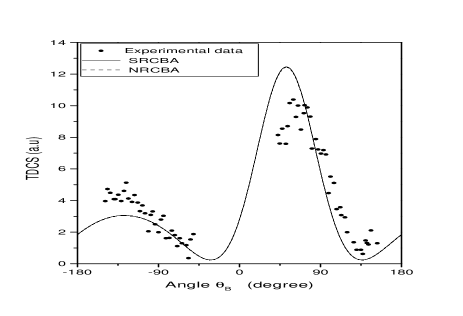
Figure 1: The two TDCSs. The solid line represents the relativistic TDCS in the semi-relativistic Coulomb Born approximation, the long-dashed line represents the corresponding TDCS in the non relativistic Coulomb Born approximation. The incident electron kinetic energy is $T_{i}=250\quad eV$ and the ejected electron kinetic energy is $T_{B}=5\quad eV$. Experimental data is from 24

.

All these results are obtained in the coplanar asymmetric geometry. Let us consider the process whereby an incident electron with a kinetic energy $E_{i}=250\text{ }eV$ scatters with a hydrogen atom. The ejected electron is observed to have a kinetic energy $E_{B}=5\text{ }eV$ and the scattered electron is observed having an angle $\theta_{f}=3$. In this particular case, the CBA is not as accurate as the results obtained within the framework of the Eikonal Born series [17] which contains higher order corrections.

Nevertheless, as it can be seen in Fig. 1, the agreement between the non relativistic and semi-relativistic results is good since we obtain two identical curves.

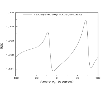
Figure 2: The ratio $TDCS(SRCBA)/TDCS(NRCBA)$ as function of the angle $\theta_{B}$ with $\theta_{f}=3^{\circ}$. The incident electron kinetic energy is $T_{i}=250\quad eV$ and the ejected electron kinetic energy is $T_{B}=5\quad eV$

.

However, even in this non relativistic regime, small effects due to the semi-relativistic treatment of the wave functions we have used, show that there are indeed small effects that can only be tracked back to the spin. Indeed, if we plot the ratio of the semi-relativistic TDCS and the non relativistic TDCS, it emerges that however small, these spin effects can reach $0,45\%$ for some specific angles. We recall that the TDCS has extrema, in particular when the direction of $\mathbf{p_{B}}$ coincides with that of the vectors $\mathbf{\Delta}$ and $-\mathbf{\Delta}$ and this can be seen in Fig. 2.

In the former case, the extremum is always a maximum and in the latter case the extremum is a local maximum. The two TDCSs exhibit in this geometry a forward or binary peak with a maximum in the direction of $\mathbf{\Delta}$ and a recoil or backward peak in the opposite direction $-\mathbf{\Delta}$. The locations of such extrema are $\theta_{B}\approx-128^{\circ}$ with a ratio equal to $1.00234$ and $\theta_{B}\approx 52^{\circ}$ with a ratio equal to $1.00185$. These mechanisms for the emergence of the binary-recoil peak structure are also present even when one uses the simplest description in which plane waves for incoming and outgoing particles are assumed [22].

Now, if we compare our result with the result obtained by Berakdar [21], we also obtain a good agreement. But before beginning the discussion proper, let us recall the formalism used by Berakdar. His calculations were performed within a model where the three-body final state is described by a product of three symmetrical, Coulomb-type functions. Each of these functions describes the motion of a particular two-body subsystem in the presence of a third charged particle. Thereafter, he made a comprehensive comparison with available experimental data and with other theoretical models. He ended his study by concluding that generally, good agreement is found with the absolute measurements but that however, in some cases discrepancies between various theoretical predictions and experimental findings are obvious, which highlights the need for a theoretical and experimental benchmark study of these reactions.

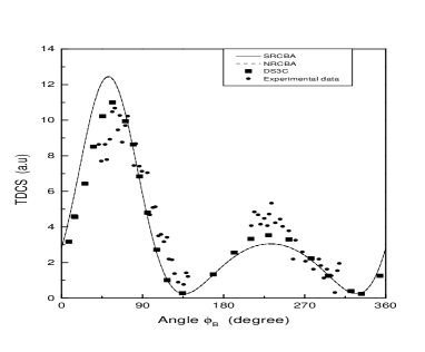
Figure 3: The two TDCSs. The solid line represents the relativistic TDCS in the semi-relativistic Coulomb Born approximation, the long-dashed line represents the corresponding TDCS in the non relativistic Coulomb Born approximation, the symbols square and circle respectively represent the formalism of DS3C and the experimental data. We keep the same energies as in Fig. 1. Experimental data is from 9

.

In Fig. 3, we compare our results with those obtained by Berakdar for an incident electron kinetic energy $E_{i}=250\text{ }eV$ for the case of a coplanar asymmetric geometric where $\theta_{f}=\theta_{B}=90^{\circ}$. The ejected electron kinetic energy is $E_{B}=5\text{ }eV$ and $\phi_{f}=357^{\circ}$. What is remarkable is the agreement between our results and his bearing in mind that he used the DS3C formalism (DS3C stands for dynamical screening theory with three Coulomb-type functions). Another atypical result related to our calculations is the behavior of the ratio of the $TDCS(SRCBA)/TDCS(NRCBA)$ where now the maxima of this ratio correspond nearly to the local minima of the TDCS when plotted as a function of the angle $\phi_{B}$.

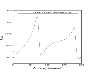
Figure 4: The ratio $TDCS(SRCBA)/TDCS(NRCBA)$ as function of the angle $\theta_{B}$ with $\theta_{f}=357^{\circ}$. The incident electron kinetic energy is $T_{i}=250\quad eV$ and the ejected electron kinetic energy is $T_{B}=5\quad eV$

.

This is shown in Fig 4. However, there is no rule that can be inferred from the behavior of this ratio since when performing various simulations even in the coplanar asymmetric geometry but with increasing values of the incident electron kinetic energy, there are many regions not close to the binary or secondary peaks that present maxima or minima.

III.2 Binary coplanar geometries

The relativistic regime can be defined as follows : when the value of the relativistic parameter $\gamma=(1-(\beta/c)^{2})^{-1/2}$ is greater that $1.0053$, there begins to be a difference between the non relativistic kinetic energy and the relativistic kinetic energy.

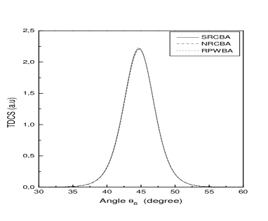
Figure 5: The three TDCSs scaled in $10^{-3}$. The solid line represents the relativistic TDCS in the semi-relativistic Coulomb Born approximation, the long-dashed line represents the corresponding TDCS in the non relativistic Coulomb Born approximation. The short-dashed line represents the rlativistic plane wave Born approximation. The incident electron kinetic energy is $T_{i}=2700\quad eV$ and the ejected electron kinetic energy is $T_{B}=1349.5\quad eV$ and $\theta_{f}=45^{\circ}$

.

This numerical value of the aforementioned relativistic parameter corresponds to an incident electron kinetic energy of $E_{i}=2700\text{ }eV$. Because there is no experimental data available for this regime, we simply compare our results with those we have previously found when we introduced the RPWBA 23 (relativistic plane wave Born approximation)to study the ionization of atomic hydrogen by electron impact in the binary geometry. In Fig. 5, it is clearly visible that the three models (NRCBA, SRCBA and RPWBA) give the same results which was to be expected since in this geometry, the use of a Coulomb wave function is not necessary.

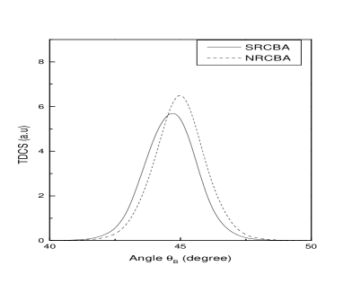
Figure 6: The two TDCSs scaled in $10^{-5}$. The solid line represents the relativistic TDCS in the semi-relativistic Coulomb Born approximation, the long-dashed line represents the corresponding TDCS in the non relativistic Coulomb Born approximation. The incident electron kinetic energy is $T_{i}=25000\quad eV$ and the ejected electron kinetic energy is $T_{B}=12499.5\quad eV$ and $\theta_{f}=45^{\circ}$

.

In Fig. 6, there is a shift of the maximum of the TDCS in the SRCBA towards smaller values than $\theta_{B}=45^{\circ}$ and this remains the case for increasing values of the kinetic energy of the incident electron. The origin of this shift stems from the fact that the main contribution to the TDCS comes from the term $H_{1}(q)$ given by Eq. (16). This term contains a dominant integral $I_{1}$. When plotting the behavior of $I_{1}$ as function of the angle $\theta_{B}$, and with increasing values of $E_{i}$, one observes the shift we have mentioned as well as the fact that in the relativistic regime, the TDCS(SRCBA) is always lower than the TDCS(NRCBA).

IV Conclusion

In this work, we have developed an exact semi-relativistic model in the first Born approximation that is valid for a wide range of geometries, simple in its mathematical structure and that allows to find previous results using sophisticated non-relativistic models. This model gives good results if the condition $Z\alpha\ll 1$ is fulfilled.

Appendix A Analytical calculation of the integral $J(\lambda)$

Before turning to the analytical calculation of the integral $J(\lambda)$ proper, let us recall how the integral $I(\lambda)$ [16] can be obtained. This is explained without any detail in [20]. Using parabolic coordinates, one has to evaluate the following integral

$$I(\lambda) = \int d\mathbf{r}\exp(i\mathbf{Q.r})\exp(-i\mathbf{p}_{B}.\mathbf{r})\frac{e^{-\lambda r}}{r}$$ (46)

$$\times {}_{1}F_{1}(i\eta_{B},1,i(p_{B}r+\mathbf{p}_{B}.\mathbf{r}))$$

The choice of the scalar product $\mathbf{Q.r}$ chosen is [6]

$$\mathbf{Q.r=}\frac{1}{2}Q(\xi-\eta)\cos\gamma-4\sqrt{\xi\eta}\cos\varphi\sin\gamma$$ (47)

Performing the various integrals, one finds

$$I(\lambda) = \frac{2\pi}{\lambda-i(Q\cos\gamma+p_{B})}\int_{0}^{\infty}d\xi\exp(-\mu\xi)$$ (48)

$$\times {}_{1}F_{1}(i\eta_{B},1,ip_{B}\xi)$$

We use the well known result [20]

$$\int_{0}^{\infty}dt\exp(-\lambda t)_{1}F_{1}(\alpha,1,kt)=\lambda^{\alpha-1}(\lambda-k)^{-\alpha}$$ (49)

with

$$\lambda=\mu=\frac{Q^{2}\sin^{2}\gamma}{2[\lambda-i(Q\cos\gamma+p_{B})]}+\frac{1}{2}[\lambda+i(Q\cos\gamma+p_{B})]$$ (50)

and $\alpha=i\eta_{B}$ and $k=ip_{B}$. This gives the result :

$$I(\lambda)=\frac{4\pi}{(Q^{2}+\lambda^{2}+p_{B}^{2}+2Qp_{B}\cos\gamma)}$$ (51)

$$\times \exp\left[i\eta_{B}\ln(\frac{Q^{2}+\lambda^{2}+p_{B}^{2}+2Qp_{B}\cos\gamma}{Q^{2}+\lambda^{2}-p_{B}^{2}-2i\lambda p_{B}})\right]$$

To recover the integral $I(\lambda)$ given in EQ. (19) of the text, one has to make the following substitutions :

$$\left.\begin{array}[]{c}-\mathbf{Q}=\mathbf{q}+\mathbf{p}_{B}\\ Qp_{B}\cos\gamma=\mathbf{Q.p}_{B}=-\mathbf{q.p}_{B}-p_{B}^{2}\end{array}\right.$$ (52)

It is then straightforward to find that

$$\left.\begin{array}[]{c}Q^{2}+\lambda^{2}+p_{B}^{2}+2Qp_{B}\cos\gamma=q^{2}+\lambda^{2}\\ Q^{2}+\lambda^{2}-p_{B}^{2}-2i\lambda p_{B}=q^{2}+\lambda^{2}+2\mathbf{q.p}_{B}-2i\lambda p_{B}\end{array}\right.$$ (53)

so that

$$I(\lambda)=\frac{4\pi}{(q^{2}+\lambda^{2})}\exp\left[i\eta_{B}\ln(\frac{q^{2}+\lambda^{2}}{q^{2}+\lambda^{2}+2\mathbf{q.p}_{B}-2i\lambda p_{B}})\right]$$ (54)

To calculate

$$J(\lambda) = \int d\mathbf{r}\exp(i\mathbf{Q.r})\exp(-i\mathbf{p}_{B}.\mathbf{r})\frac{e^{-\lambda r}}{r}$$ (55)

$$\times \text{ }_{1}F_{1}(i\eta_{B}+1,2,i(p_{B}r+\mathbf{p}_{B}.\mathbf{r}))$$

one uses the same procedures to obtain

$$J(\lambda) = \frac{2\pi}{\lambda-i(Q\cos\gamma+p_{B})}\int_{0}^{\infty}d\xi\exp(-\mu\xi)$$ (56)

$$\times {}_{1}F_{1}(i\eta_{B}+1,2,ip_{B}\xi)$$

$$= \frac{2\pi}{\lambda-i(Q\cos\gamma+p_{B})}\frac{1}{\mu}$$

$$\times {}_{2}F_{{}_{1}}(i\eta_{B}+1,1,2,\frac{ip_{B}}{\mu})$$

Performing the various substitutions, one gets the following new (as far as we know) analytical integral

$$J(\lambda)=\int d\mathbf{r}\exp(i\mathbf{q.r})\frac{e^{-\lambda r}}{r}\,_{1}F_{1}(i\eta_{B}+1,2,i(p_{B}r+\mathbf{p}_{B}.\mathbf{r}))=\frac{4\pi}{(q^{2}+\lambda^{2})}\text{ }_{2}F_{1}\left(i\eta_{B}+1,1,2,-2\frac{[\mathbf{q.p}_{B}-i\lambda p_{B}]}{q^{2}+\lambda^{2}}\right)$$ (57)

We have tested this analytical result by performing the integral using two gaussian quadratures because we have assumed without loss of generality both $\mathbf{q}$ and $\mathbf{p}_{B}$ to be parrallel to the $Oz$ axis. The first one, a Laguerre gaussian quadrature (32 points) to integrate over the radial variable $r$ and the second one, using a Legendre gaussian quadrature (32 points) to integrate over the angular variable $\theta$. The agreement between the analytical result and the numerical result is excellent. To illustrate this point, we give as an exemple the results obtained by the two methods for the following random values of the relevant parameters. For $\lambda=1$ ,$\left|\mathbf{q}\right|$=1.015055, $\left|\mathbf{p}\right|=$0.1055098. The exact result is

$$J_{exact}(\lambda)=(0.57355896,0.12458510)$$ (58)

and the numerical result is :

$$J_{num}(\lambda)=(0.57355899,0.12458507)$$ (59)

References

- (1) W. Nakel and C.T. Whelan, Phys. Rep., 315, 409, (1999).
- (2) C .T. Whelan, R.J. Allan, J. Rasch, H.R.J. Walters, X. Zhang, J. Röder, K. Jung, H. Ehrhardt, Phys. Rev A, 50, 4394, (1994).
- (3) P. Marchalant, C.T. Whelan, H.R.J. Walters, J. Phys. B, 31, 1141, (1998).
- (4) I. Fuss, J. Mitroy, B.M. Spicer, J. Phys. B, 15, 3321, (1982).
- (5) I.E. McCarthy, E. Weigold, Cont. Phys., 35, 377, (1994).
- (6) F. Bell, J. Phys. B, 22, 287, (1989).
- (7) A. Cavaldi, L. Avaldi, Nuovo Cimento Soc. Ital. Fis., D 16, 1, (1994).
- (8) H. Ehrhardt, Comments At. Mol. Phys., 13, 115, (1983).
- (9) H. Ehrhardt, K. Jung, G. Knöth, P. Schlemmer, Z. Phys., D 1, 3, (1986).
- (10) J.N. Das, A.N. Konar, J. Phys. B, 7, 2417, (1974).
- (11) J.N. Das, S. Chakraborty, Phys. Lett. A, 92, 127, (1982).
- (12) B.L. Moïseiwitsch, Prog. At. Mol. Phys., 16, 281, (1980).
- (13) D.H. Jakubaßa-Amundsen, Z. Phys., D 11, 305, (1989).
- (14) D.H. Jakubaßa-Amundsen, Phys. Rev A, 53, 2359, (1996).
- (15) L.U. Ancarani, S. Keller, H. Ast, C.T. Whelan, H.R.J. Walters, R.M. Dreizler, J. Phys. B, 31, 609, (1998).
- (16) H.S.W. Massey and C.B.O Mohr, Proc. Roy. Soc. A 140, 613, (1933)
- (17) F.W. Jr Byron and C.J. Joachain, Phys. Rep. 179, 211, (1989).
- (18) J. Eichler and W.E. Meyerhof, Relativistic Atomic Collisions, Academic Press, (1995).
- (19) W. Greiner and J. Reinhardt, Quantum Electrodynamics, Springer-Verlag, (1992).
- (20) L. Landau and E. Lifchitz, Mécanique quantique, Editions Mir, Moscou, (1967).
- (21) J. Berakdar, Phys. Rev A, 56, 370, (1997).
- (22) J.S. Briggs, Comments At. Mol. Phys., 23, 155, (1989).
- (23) Y. Attaourti and S. Taj, Phys. Rev. A 69, 063411 (2004).
- (24) H. Ehrhardt, G. Knoth, P. Schlemmer and K. Jung, Phys. Lett. A 110, 92, (1985).