Updating Seismic Hazard at Parkfield

Abstract

The occurrence of the September 28, 2004 $M_{w}$=6.0 mainshock at Parkfield, California, has significantly increased the mean and aperiodicity of the series of time intervals between mainshocks in this segment of the San Andreas fault. We use five different statistical distributions as renewal models to fit this new series and to estimate the time-dependent probability of the next Parkfield mainshock. Three of these distributions (lognormal, gamma and Weibull) are frequently used in reliability and time-to-failure problems. The other two come from physically-based models of earthquake recurrence (the Brownian Passage Time Model and the Minimalist Model). The differences resulting from these five renewal models are emphasized.

guessConjecture

1 Introduction

Renewal models are frequently used to estimate the long-term time-dependent probability of the next large earthquake on specific faults or fault segments where large shocks occur repeatedly at approximately regular intervals. In this approach, it is assumed that the times between consecutive large earthquakes (inter-event times or recurrence intervals) follow a certain statistical distribution. The available record of large earthquakes in any given fault is typically scarce (usually including less than ten events), so the empirical statistics are poor. Because of this, a theoretical distribution is fitted to the observed inter-event times and used to estimate future earthquake probabilities. In the first instance, several well-known statistical distributions were used [Utsu (1984), Ellsworth et al. (1999)]. These distributions have only an empirical rooting and are commonly employed as renewal models in reliability and time-to-failure problems [Ellsworth et al. (1999)]. Three of these distributions (the gamma, lognormal, and Weibull) are frequently used for earthquakes, because they share three properties commonly observed for earthquake inter-event times [Michael (2005)]: First, these times must be positive, and these distributions only exist for positive times; second, inter-event times much smaller than the average recurrence interval are rare; and third, the distribution of inter-event times decays slowly for times longer than the average.

More recently, the distributions derived from two simple physical models of earthquake recurrence have been proposed as an alternative to those purely empirical approaches. These two models have the virtue of providing an intuitive picture of the seismic cycle in a fault or fault segment. They are the Brownian Passage Time Model [Kagan and Knopoff (1987), Ellsworth et al. (1999), Matthews et al. (2002), WGCEP (2003)], and the Minimalist Model [Vázquez-Prada et al. (2002), Gómez and Pacheco (2004)]. The first one represents the tectonic loading of a fault by a variable which evolves by superposition of an increasing linear trend and a Brownian noise term, and an earthquake occurs when this variable reaches a given threshold [Matthews et al. (2002)]. All the earthquakes in this model are identical to each other. The Minimalist Model sketches the plane of a seismic fault, where earthquake ruptures start and propagate according to simplified breaking rules. This model generates earthquakes of various sizes, and only the time between the largest ones (the characteristic earthquakes, that break the whole model fault) are considered for the inter-event time distribution. The distributions derived from these two models, as well as the gamma, lognormal and Weibull, generally represent fairly well the observed distribution of large-earthquake inter-event times [Gómez and Pacheco (2004)]. However, they differ significantly in their probability predictions for times much longer than the mean inter-event time of the data. Thus, it seems convenient to take all their different predictions into account.

The paucity of data in the record of large earthquakes in a given fault or fault segment has another consequence. The occurrence of a new large shock significantly modifies the mean and aperiodicity of the available series of inter-event times. In turn, this significantly modifies the parameters of the best fit of the statistical distribution used for the adjustment, resulting in different estimations of future earthquake probabilities. Thus, for seismic hazard assessment, it is important to recalculate the new parameters. This is just the case at the Parkfield segment of the San Andreas fault in California with the September 28, 2004, $M_{w}=6.0$ earthquake, which significantly increased both the mean and the aperiodicity of the available series. Therefore, the purpose of this short communication is to update the previous fits [Ellsworth et al. (1999), Gómez and Pacheco (2004)] to this new series and compare the hazard predictions coming from five different renewal models: the gamma (G), lognormal (LN) and Weibull (W) distributions as classical renewal models, and also the Brownian Passage Time Model (BPT) and the Minimalist Model (MM), as more recent counterparts.

In Section II, the mean and the aperiodicity of the new series are calculated. Besides, this section contains the best fits obtained by the method of moments with the different renewal models. Finally, in Section III we discuss the probability estimates for the next mainshock at Parkfield.

2 Fits to the new series

Including the latest event, the Parkfield series [Bakun and Lindh (1985), Bakun (1988), Michael and Jones (1998)] consists of seven $M_{w}\simeq 6$ mainshocks, which occurred on January 9, 1857; February 2, 1881; March 3, 1901; March 10, 1922; June 8, 1934; June 28, 1966 and September 28, 2004. In consequence, the duration (in years) of the six observed inter-event times are: 24.07, 20.08, 21.02, 12.25, 32.05 and 38.25. The mean value $m$, the sample standard deviation $s$ (the square root of the bias-corrected sample variance), and the aperiodicity $\alpha$ (equivalent to the coefficient of variation, i.e. the standard deviation divided by the mean) of this six-data series are:

$$m=24.62\mbox{ yr}\qquad s=9.25\mbox{ yr}\qquad\alpha=0.3759$$ (1)

Now, we will proceed to fit these data using the G, LN and W families of distributions [Utsu (1984)] and the BPT and MM models [Matthews et al. (2002), Gómez and Pacheco (2004)]. The statistical distribution of inter-event times in the BPT model is the so-called inverse Gaussian distribution, which, as the three classical distributions mentioned at the beginning, is a continuum biparametric density distribution. Strictly speaking, the distribution derived from the MM is a discrete one and has only one parameter, $N$ (the number of cells in which the model fault plane is divided, directly related to the aperiodicity $\alpha$ of the series) [Gómez and Pacheco (2004)]. However, for fitting the data, it is necessary to assign a definite number of years to the non-dimensional time step of the model. This second parameter will be called $\tau$. The distribution in the MM has an analytical solution, explicitly written for $N\leq 5$ in Gómez and Pacheco (2004). For larger values of $N$ the distribution can be calculated numerically with Monte Carlo simulations.

Next, we will write down the explicit analytic form of the four mentioned continuum probability density distributions. Each of them has a scale parameter and a shape parameter. In all formulae the time, $t$, is measured in years.

Gamma distribution:

$$G(t)=\frac{c}{\Gamma(r)}(ct)^{r-1}e^{-ct},\quad c>0,\;r>0$$ (2)

Lognormal distribution:

$$LN(t)=\frac{1}{\sqrt{2\pi}\sigma t}\exp\left[-\frac{(\ln t-n)^{2}}{2\sigma^{2}}\right],\qquad n>0,\;\sigma>0$$ (3)

Weibull distribution:

$$W(t)=a\rho t^{\rho-1}\exp(-at^{\rho}),\qquad a>0,\;\rho>0$$ (4)

Brownian Passage Time distribution Matthews et al. (2002):

$$BPT(t)=\left(\frac{m}{2\pi\alpha^{2}t^{3}}\right)^{1/2}\exp\left[-\frac{(t-m)^{2}}{2m\alpha^{2}t}\right]$$ (5)

In this last case, the parameters $m$ and $\alpha$ correspond to the mean and aperiodicity defined earlier.

We will use the method of moments to fit the data, so within these four families of distributions, and the same for the MM, we will select that specific distribution whose mean value and aperiodicity are equal to those of the Parkfield series (Eq. 1). The specific values of the parameters that make the different distributions fulfill this condition are written in Table 1.

Gamma	$c=0.287\;yr^{-1}\quad r=7.078$
Lognormal	$n=3.137\quad\sigma=0.364$
Weibull	$a=6.853\times 10^{-5}\;yr^{-\rho}\quad\rho=2.889$
BPT	$m=24.62\;yr\quad\alpha=0.3759$
MM	$N=495\quad(\alpha=0.3759)\quad\tau=4.186\times 10^{-3}\;yr$

Table 1: Parameter values obtained by the method of moments for the five renewal models described in the text for the Parkfield series.

Note that in the MM model the aperiodicity of the series fixes the value of the parameter $N$ Gómez and Pacheco (2004). In a minimalist system with $N=495$, the mean recurrence interval of the characteristic earthquakes is 5881.2 non-dimensional time steps. Comparing this mean with the value $m=24.62$ yr quoted in Eq. 1, we deduce that one time step of the model corresponds to $\tau=24.62$ yr$/5881.2=4.186\times 10^{-3}$ yr, or around 1.5 days.

In Fig. 1a, we have superimposed the cumulative histogram (empirical distribution function) of the Parkfield series together with the cumulative distributions of the five models. These, for the G, LN, W and BPT are obtained by integrating Eqs. 2-5, and for the MM by summing its discrete probability distribution. In Fig. 1b we show the residuals for the five fits. Finally, in Fig. 2 we present the annual (conditional) probability of occurrence derived from the five models Utsu (1984).

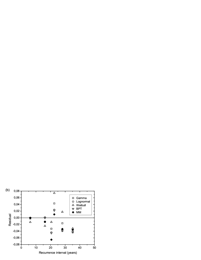
Figure 1: Comparison of the performance of different renewal models. (a) Fit to the Parkfield sequence of the gamma, lognormal, Weibull, BPT and MM models; (b) residuals for the five model fits, evaluated at the midpoints of the horizontal segments of the empirical distribution function.

Figure 2: Annual probability for the new mainshock at Parkfield according to the five renewal models.

3 Discussion and conclusions

The results shown in Fig. 1a and 1b indicate that the five models used in the adjustment describe rather well the Parkfield data, despite being different from each other. All the residuals (Fig. 1b) are lower than 8% at any time (most of them lower than 4%). The minimum residual is not always related to the same model, and the ‘best’ model changes with time. This precludes selecting one particular model as the optimal choice for prediction purposes.

It is clear from Fig. 1a that the curve corresponding to the MM takes off later than the others. This is because in this model there exists an initial stress shadow with a length of $N=495$ time steps, i.e. $495\times 4.186\times 10^{-3}$ yr, that is 2.07 yr. Thus, in this model, in the initial 2.07 yr of the cycle definitely no new event can occur. This is in stark contrast to the other renewal models, where there is no strict stress shadow. Most distributions have a low or very low probability of occurrence between 0 an 2.07 yr, but none have a strictly zero probability as the MM has. The LN and BPT curves plot one upon the other in Fig. 1a because in the time range shown in the graph their cumulative probability distributions are similar. Note also that the Weibull model predicts a cumulative probability considerably higher for $t<10$ yr than the other four models, and that all five cumulative distribution functions appear to ‘converge’ in probability roughly 18 yr after the last mainshock, with a cumulative probability of around 25%. All the models indicate that an immediate rerupture of the Parkfield segment is unlikely (the cumulative probabilities are lesser than 1% for the first five years), but it will likely occur not later than 53 years after the last one (moment at which all cumulative probabilities are at least 99%).

In Fig. 2, where the annual probability of occurrence is shown, there are several observations worth comment. At the beginning of the cycle the W curve is the first in the take off and the MM is the last. This reflects what was mentioned in the previous paragraph. Later, there is an interval, roughly speaking from 2016 to 2023, in which the MM curve is on top of the others, predicting slightly higher annual probabilities. Around 2030, when the mean recurrence interval of the series has elapsed, all the models predict a yearly conditional probability between 8.5% and 10%. The predictions from the LN and the BPT are very similar until about 2040, because the BPT distribution is similar to, but not identical to, a lognormal distribution Michael (2005). But from 2040 onwards, the five models start showing their asymptotic behaviour, or, in other words, their clear discrepancies. The behaviour of the conditional probability for long times after a large earthquake is still debated (e.g. Davis et al. 1989; Sornette and Knopoff, 1997), and the different models used in this paper show three different possibilities for it. First, a decreasing probability, the case of the LN model, where the probability starts declining from the year 2053 onwards, approaching zero as time passes. Second, a probability which increases asymptotically to 100%, the case of the W model, according to which there is a 95% yearly probability of having a mainshock after 163 yr from the last one. And third, a probability that increases towards an asymptote smaller than 100%, the case of the curves predicted by the BPT, G and MM models. The asymptotic yearly probability value is different for each of these three models: 13%, 26%, and 38% respectively. This last value in the MM is given by the formula

$$\lim_{n\to\infty}P(n,\tau)=\frac{N-1}{N}\left[1-\left(\frac{N-1}{N}\right)^{\frac{1}{\tau}}\right],$$ (6)

where $n$ is the number of time steps since the last characteristic earthquake in the model.

The discrepancies between the predictions of these five approaches cannot be used to disregard any of them, at least for the first decades since the last mainshock. On the contrary, they can be considered all together to give reasonable upper and lower bounds to the annual probability of occurrence at Parkfield: between 8.5% and 10% after 25 yr (i.e., after one mean cycle length), and between 12% and 17% after 37 yr (i.e., after 1.5 mean cycle lengths).