Study of charge-charge coupling effects on dipole emitter relaxation within a classical electron-ion plasma description

Abstract

Studies of charge-charge (ion-ion, ion-electron, and electron-electron) coupling properties for ion impurities in an electron gas and for a two component plasma are carried out on the basis of a regularized electron-ion potential without short-range Coulomb divergence. This work is motivated in part by questions arising from recent spectroscopic measurements revealing discrepancies with present theoretical descriptions. Many of the current radiative property models for plasmas include only single electron-emitter collisions and neglect some or all charge-charge interactions. A molecular dynamics simulation of dipole relaxation is proposed here to allow proper account of many electron-emitter interactions and all charge-charge couplings. As illustrations, molecular dynamics simulations are reported for the cases of a single ion imbedded in an electron plasma and for a two-component ion-electron plasma. Ion-ion, electron-ion, and electron-electron coupling effects are discussed for hydrogen-like Balmer alpha lines.

I Introduction

Theories for the interpretation of spectroscopic measurements in hot plasmas are crucial for diagnosing and studying laboratory and astrophysical plasmas. Well known theories such as the impact theory impact or the unified theory unified for electron broadening will be mentioned below. It should be emphasized that in this context a “theory” is a closed ensemble of many theoretical developments built on the basis of an initial set of hypotheses, namely a “model” (possibly including a few variants). Within each theory, specific analytical and numerical methods are assumed for practical calculation of the physical properties that belong to that theory. The analysis here addresses the validity of common assumptions regarding the many-body Coulomb forces for computing radiative properties. More specifically, the lineshapes of ion emitters in fully ionized plasmas are investigated using classical molecular dynamics (MD) simulation. The advantage of MD simulation lies in its ability to account for all charge-charge interactions without approximation, providing a means to assess their relative importance for lineshape calculations.

Most of the current models for the study of radiative properties of an emitter in a dilute medium treat the internal states of the emitter quantum mechanically, but use a semi-classical description for their interaction with the environment for the description of the environment. The system considered here is the same: a quantum emitter of charge $Ze$ imbedded in an equilibrium classical plasma with ions of charge $Z_{i}e$ and electrons of charge $-e$ at equilibrium. For simplicity, in all of the following it is assumed that the emitter couples to the plasma only through its monopole and dipole interactions.

The line shape is then determined by the Stark broadening of the total electric field at the emitter. Three timescales have to be considered together: those characterizing ion motion, $\tau_{i}$, electron motion, $\tau_{e}$ and a typical emitter dipole relaxation time, $\tau_{d}$. In all cases $\tau_{i}$ is much larger than $\tau_{e}$ due to their large mass ratio. Consequently, the ions do not respond directly to individual electron motions but rather to their averaged collective dynamics whose primary effect is to screen the ion-ion interactions. Conversely, the free electrons are coupled to all other electrons, and a slowly varying ion and emitter charge distribution through unscreened potentials. Similarly, the optical electrons bound to the emitter and responsible for radiation emission are coupled to the classical charges through a slowly varying screened ion field, and rapidly varying electric fields due to the colliding electrons via the dipole interaction. In some current theories the effects of this complex plasma environment are represented through the hypothesis of atomic or ionic emitters interacting with ions through a Coulomb field screened at the electronic Debye length and by free electrons moving on straight trajectories (no electron-emitter or electron-electron interactions) - hereafter called independent-electrons. The simplest formulation of the impact theory for electron broadening is developed on this basis with three additional constraints for the independent electrons: 1) non-overlapping strong collisions (binary collision approximation), 2) positive lower bound for the impact parameter range (strong collision cut-off), and 3) a Debye screened Coulomb interaction between free and bound emitter electrons. In such theories, collective effects or correlations among the various charges are accounted for only in the static Debye screened ion-emitter and electron-emitter fields. The objective of our presentation here is to explore in a controlled fashion the effects of correlations, both static and dynamic, on properties relevant to plasma spectroscopy.

Lineshape calculations follow two distinct stages: first, the “stochastic” properties of the local electric field perturbation at the charged emitter from a classical plasma model are determined, and next these properties are used for modeling the dipole emission. The first point refers to a determination of charge structure and dynamics, and is essentially a nonlinear problem depending on the emitter monopole charge and the plasma parameters - a plasma physics problem. The second is connected to the behavior of a quantum emitter in a given time dependant stochastic perturbation - an atomic physics problem. The utility of MD simulation to treat the plasma physics component “without approximation” is well-known plasmaMD , although the application to study correlation effects of electrons with higher $Z$ ions is a new direction for hot plasmas tal1 . However, in order to assess the importance of such effects for spectroscopy, the atomic physics component is essential. The results presented here are a first attempt to combine MD simulation and atomic physics for a controlled description of both electron and ion broadening tal2 . Earlier applications of MD to spectral line broadening were limited to simulating the plasma ion fields ionMD . Here, we emphasize the more difficult task of simulating as well the electrons which couple to the emitter in a qualitatively different way due to their attractive interaction.

The classical plasmas considered for simulation are systems of point charges, either point electrons and the emitter monopole in a uniform positive background - hereafter called inhomogeneous jellium - or a two component plasma (TCP) of electrons plus the emitter monopoles. It is assumed that quantum mechanical effects are either negligible (as for the heavy ions and emitter) or can be incorporated through appropriate modifications of the classical Coulomb potential for the electrons. The latter is achieved by using a regularized Coulomb potential which remains finite at short distances, accounting simply for the true quantum diffraction effects Minoo . This allows derivation of all the desired theoretical properties using the laws of classical mechanics, as well as the application of MD. A detailed study of the time independent statistical properties of an electron gas with an ion impurity has been carried out recently on the basis of such a regularized electron-ion potential tal1 . Two standard classical methods have been used for this study: molecular dynamics (MD) for numerical simulation for both dynamical and structural properties, and the hypernetted chain approximation (HNC) for the theoretical prediction of structural properties. This enables both cross comparisons and interpretations of results. An interpretation of the dynamical properties of the electron field autocorrelation function (FCF) at the impurity also has been carried out dufty-ilya and is considered further here.

Molecular dynamics is a unique way for providing realistic representations of the stochastic electric fields determining the dipole interaction of the emitter with its environment. Describing these fields by simulation allows one to obtain lineshapes accounting for all the correlations between charged particles. Such lineshapes would provide essential reference data to benchmark more efficient but phenomenological theoretical models developed for plasma diagnostics. Several recent theories for line broadening have been developed for investigations at new plasma conditions, including the hot and dense matter conditions needed for the presence of highly charged emitters. They suggest that part of the discrepancies found with experiments is an inadequate description of the emitter and electron perturber coupling mechanisms. The present study provides new information for this discussion.

The types of questions posed are the following: 1) What is the validity of straight line trajectories for the electrons in the presence of a charged emitter (neglect of electron-emitter, electron-electron, and electron-ion coupling in the dynamics)? 2) How well are the missing correlations of 1) captured by simple screening of the electron emitter interaction? 3) What is the importance of multi-electron strong collisions? This study addresses these issues for two different classical plasma environments of the emitter. Both are well distinct from those resulting from independent electron models assumed for impact theories. The first and simplest is the inhomogeneous jellium used for describing electron broadening only. The corresponding study is hereafter referred to as the electron broadening theory (EBT). The second is a more realistic two component electron-ion plasma leading to a both ion and electron broadening theory (IEBT). The parameter range explored in this work is chosen to be compatible with hot and dense plasma diagnostics based on spectroscopy. These are conditions similar to those for which there are long standing discrepancies between theory and experiment. For a recent discussion and earlier references see reference 3s3p .

In section II the main points of the classical plasma study for the positive charge emitter in the above two plasma environments is described. Section III outlines the dipole relaxation stage of the broadening theories reported in this paper. Then, the main results obtained with the EBT, i.e. the effects of ion-electron correlations on electron broadening of spectral lines, are reported and discussed. Also in Section III dipole relaxation in a TCP is considered and some preliminary results obtained using the the IEBT are shown. The examples reported below involve the Balmer alpha line for various hydrogen-like emitters of charge 1, 3, 5 and 8 and various temperatures.

II Plasma environment modeling

This section provides an illustration of the results that can be obtained from MD simulation for the two types of plasma environments considered for the emitter. In both the inhomogeneous jellium and the two component electron-ion plasma (TCP), the monopole of the emitter is included as a point charge. The dipole operator representing the internal states of the emitter is not considered in this section. For the density and temperature conditions considered the repulsive interactions of same sign charges effectively excludes pair configurations of the order of the DeBroglie wavelength and quantum effects are small. Consequently, the ion-ion, ion-emitter, and electron-electron interactions are taken to be Coulomb

$$V_{12}(r)=Z_{1}Z_{2}e^{-r/\lambda}/r$$ (1)

where $Z_{1}Z_{2}$ is positive. For practical purposes these Coulomb interactions have been screened at a distance $\lambda=s/2$ which is taken to be of the order of the system size $s$. This allows application of the usual periodic boundary conditions in the MD simulation. Since interactions among the charges introduce a physical screening at much shorter distances, this system size screening does not affect any of the properties being considered here. In contrast, electron-ion and electron-emitter interactions are attractive and the configurations within a DeBroglie wavelength become relevant. At such distances the Coulomb interaction must be modified within a classical description to account for quantum diffraction effects. There are many ways such quantum potentials can be constructed and here we use one of the simplest forms Minoo

$$V_{ie}(r)=-Ze^{2}(1-e^{-r/\delta})e^{-r/\lambda}/r$$ (2)

where $\delta=(2\pi\hbar^{2}/m_{e}k_{B}T_{e})^{1/2}$ is the thermal De Broglie wavelength. This ion-electron potential regularization provides a well defined classical physics for opposite sign charge systems, and the various sophisticated classical N-body methods of classical statistical mechanics can be applied. The consequences and advantages of such a semi-classical approach for the radiative properties of ion emitters will be discussed in the last sections.

Other parameters of interest are the average electron-electron distance $r_{0}=(3/4\pi N_{e})^{1/3}$ defined in terms of the electron density $N_{e}$, the electron thermal velocity $v_{0}=(2k_{B}T_{e}/m_{e})^{1/2}$, the mean electronic field $E_{0}=e/r_{0}^{2}$, the electron-electron coupling constant $\Gamma=e^{2}/r_{0}k_{B}T_{e}$, and the electron plasma frequency $\omega_{p}=(4\pi N_{e}e^{2}/m_{e})^{1/2}$. The coupling between the electrons and the impurity is measured by the ion-electron potential at the origin which, in units of $r_{0}$, becomes $\sigma=Z\Gamma/\delta$. Similar quantities are defined for the ions in the TCP by replacing the magnitude of the electron charge and density by the corresponding ion values.

Molecular dynamics simulations are carried out using a number $N$ of electrons for the jellium, or $N$ electrons and $N/Z_{i}$ ions for the TCP. In the first case a point charge ${Z\ll N}$ representing the emitter is included while for the TCP the ions are considered as the emitters for simplicity. The simulation is done using periodic boundary conditions on an elementary cubic cell of size $c$ large enough to ensure $\lambda>\lambda_{D}$, where $\lambda_{D}$ is the Debye wavelength, and $\lambda\leq s/2$. These conditions assure that the physical screening due to the charge interactions occur at a shorter scale than the system size screening, as noted above. Because $N$ must be large to agree with the condition $Z\ll N$ the impurity-impurity correlation inherent to periodic boundary conditions is negligible. Moreover as we are only interested in the charge structure and dynamics in the ion vicinity the usual Ewald’s sum is not required. Particle motion in MD simulation is achieved using a Verlet algorithm with a time step error of order $(\Delta t)^{4}$: $\mathbf{r}_{n+1}=2\mathbf{r}_{n}-\mathbf{r}_{n-1}+\mathbf{a}_{n}(\Delta t)^{2}$.

II.1 Ion emitter in an electron gas

This section summarizes the study of a single ion impurity (the monopole of the emitter) imbedded in an electron gas. A uniform positive background maintains overall charge neutrality but has no effect on particle motion since, according to periodic boundary conditions used in molecular dynamics, the charges move across an infinite system. The motivations for doing the impurity case are: 1) it is a well defined and simpler problem than the TCP case in comparison, and 2) all the existing theories for electron broadening to compare with are based on an impurity approach. The main statistical properties of the electron structure close to the ion (e.g., electron density, electric field probability distribution) are derived using both MD simulation and the classical hypernetted chain (HNC) integral equations for the impurity-electron correlation function.

Ion-electron and electron-electron coupling affect both the static and dynamic properties of the electrons near the impurity ion. The former determines the dominant $Z$ dependence of these properties, while the latter controls the screening and other quantitative effects. The electron density, electric microfield distribution, and electric field autocorrelation function have been studied for various temperatures, densities, and impurity charge number $Z$.

Consider first the electron density near the impurity. The simplest prediction is given by the Debye-Huckel approximation leading to an enhanced density near the ion and Debye screening at large distances. This approximation is expected to fail for increased electron-ion coupling (larger values of $Z$) and/or increased electron-electron coupling. In that case an adequate theory is provided by the two component HNC equations Rogers specialized for the single impurity case, i.e. for a vanishing ion density. The impurity-electron pair distribution function $g_{ie}(r)$ is obtained by numerical solution to these equations as a function of the direct electron-electron correlation function $c_{ee}(r)$ calculated separately. Aside from normalization, this pair correlation function is the average electron number density, $n_{e}\left(r\right)=n_{e}g_{ie}(r)$ at a distance $r$ from the ion. Both MD simulation and the HNC approximation are restricted to a limited range of values for the impurity charge, density, and temperature. Outside of this range frequent electron trapping and non-convergent iterative solution methods for the HNC equations occur invalidating the results. Within the parameter space considered here MD and HNC results are in good agreement as illustrated in Fig. 1.

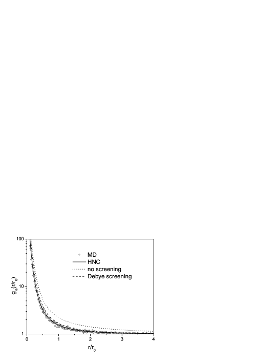
Figure 1: Ion-electron pair correlation function at $N_{e}=10^{19}cm^{-3}$, $T_{e}=50000K$, and Z=8. Solid line: HNC; circles: MD; dashed: no e-e coupling and Debye screening; dotted: no e-e coupling and no screening.

The enhanced electron accretion around the ion impurity is due to the attractive impurity-electron interaction. If this coupling is neglected the electron distribution becomes uniform regardless of the electron-electron coupling. Clearly, the independent electron model is a bad approximation for the electron density except for $Z=0$. Also shown in Fig. 1 is the result obtained by including the impurity-electron interaction but neglecting electron-electron interactions. This misses the screening effects at larger distances due to the electron coupling. For the conditions considered, the electron coupling is small, approximately $\Gamma=0.116$, and the simple addition of Debye screening gives quite good results. Other properties involving the local electron electric field at the impurity are of primary interest for spectroscopy since they determine the dipole coupling to the internal states of the emitter. The electric field for the current case is determined from the gradient of the potential in Eq. 2. For the independent electron approximation, the screening of this field is changed to the Debye length. Theoretical predictions of the electric microfield distribution can be obtained in terms of $g_{ie}(r)$ and the results using HNC have been compared with those from MD, again with good agreement. The MD results are illustrated in Fig. 2 for two values of impurity charge $Z=1$ and $Z=8$.

Figure 2: Field distribution at $N_{e}=10^{19}cm^{-3}$, $T_{e}=200000K$. Solid: $Z=1$; dashed: $Z=8$; dots: independent electrons.

The effect of increased charge number is to decrease and broaden the distribution. Also shown is the result for independent electrons. This is the $Z=0$ interaction without electron-electron interactions, but with Debye screened fields. It is seen to be similar to the $Z=1$ results. As with the average electron density, the dominant Z dependence is due to the impurity-electron coupling. However, at fixed $Z$ the electron-electron coupling is responsible for important quantitative changes in the location of the maximum and width of the distribution.

The simplest measure of the electric field dynamics is given by the field autocorrelation function (FCF). Figure 3 shows the time dependence for the cases $Z=1$ and $Z=8$ at $T_{e}=200000K$.

Figure 3: Field autocorrelation function, same as Fig. 2.

Also shown is the independent-electron limit obtained for screened fields but removing all interactions. As with the field distribution function, the result is similar to the Z=1 case. The ad hoc screening of the fields assures that the initial value is similar to that with electron-electron coupling. This screening also assures that the straight trajectory dynamics is effectively restricted to a Debye sphere. However, the electron-impurity coupling changes this agreement dramatically at larger values of $Z$. Qualitatively, the behavior of the correlation function can be summarized as follows: For increasing impurity charge number the initial value $<E^{2}>/E_{0}^{2}$ increases while the correlation time decreases. Both effects are missed by the independent electron approximation, but are regained qualitatively if only impurity-electron coupling is retained (without electron-electron interactions). However electron-electron coupling is required for quantitative effects as indicated below.

Now consider the effects of electron-electron coupling in more detail for the case $Z=1$. Figure 4 shows the results for two different temperatures, $T_{e}=200000K$ and $T_{e}=50000K$.

Figure 4: FCF for two temperatures at Z=1. Dash: no coupling; solid: all couplings.

This corresponds to two different values for the electron-electron coupling constant, $\Gamma=0.029$ and $\Gamma=0.116$, and two different values for the electron-ion coupling constant, $\sigma=0.5$ and $\sigma=1$, for the high and low temperature cases, respectively. Also shown for comparison are the results for the independent electron model. The initial value of the FCF is seen to increase at constant $Z$ for increasing temperature. This can be understood since the regularized potential leads to a covariance proportional to $1/\delta\sim{T^{1/2}}$. The correlation time decreases at higher temperatures, in part at least due to the increased thermal velocity. As expected, the deviation of the independent electron model from these results increases with increased electron coupling. The apparent agreement for the high temperature case is misleading in this presentation, since the percent discrepancies are large over the entire time interval as will be shown in Fig. 7 below. The effect of electron-electron coupling on the dynamics is therefore important. This is more evident for the lower temperature comparison.

The strong electron-impurity coupling case of $Z=8$ is shown in more detail in Fig. 5.

Figure 5: FCF anti-correlation for $Z=8$ and $T_{e}=100000K$.

A striking new feature is the anticorrelation (negative FCF) at intermediate times. This effect increases for larger $Z$ and also for decreasing temperature, corresponding to the enhanced electron–ion interactions. This increases the probability of electron configurations near the ion. Many of these lead to temporary orbiting trajectories with associated large oscillatory electric fields. When such trajectories dominate the contribution to the FCF, their changing fields on average will lead to an anticorrelation as observed in Fig. 5. The occurrence of such events is easily seen in the MD simulations, as shown in Fig. 6. The total field is dominated by the oscillatory fields of a few close orbits. These oscillations persist on the time scale of the FCF, but are seen to break up on a time scale an order of magnitude longer, due to electron-electron interactions. Thus, the effect of anticorrelation is due to quasi-bound orbits, but their correct equilibrium statistical sampling requires the electron-electron interactions to assure the properly weighted ensemble of $\it{temporary}$ orbiting trajectories.

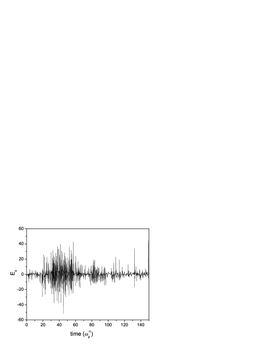
Figure 6: Example of temporarily oscillating electric field at the ion. $Z=8$ and $T_{e}=100000K$.

A general remark can be addressed about the MD approach in the context of this discussion. The field history sampling is started after a thermal equilibration stage intended to reach a stationary energy state. Independent samplings are obtained starting from a new uniform random configuration of particles followed by a thermal equilibration stage. This process is repeated many times in order to build a very large sample set. If the electron-electron coupling is neglected, the equilibration stage does not favor the electron accretion around the ion impurity in the correct way. As a result the sample set obtained is certainly not the same as the sample set obtained when the electron-electron interaction is accounted for. An improved sampling could be built using initial configurations chosen in order to agree with the nonlinear electron distribution around a positive charge. This way has been followed to develop a simple theoretical model for the FCF dufty-ilya .

It will be seen later that the spectral line width is proportional to the time integral of the FCF. It is difficult to predict the $Z$ dependence of this integral a priori due to the above competing effects of increasing initial value and decreasing correlation time. Consider again the FCF for $Z=1$ in Fig. 4 at two different temperatures. The time integral of these correlation functions and another at $100000K$ are shown as a function of temperature in Fig. 7. Also shown are the corresponding results for the independent particle model.

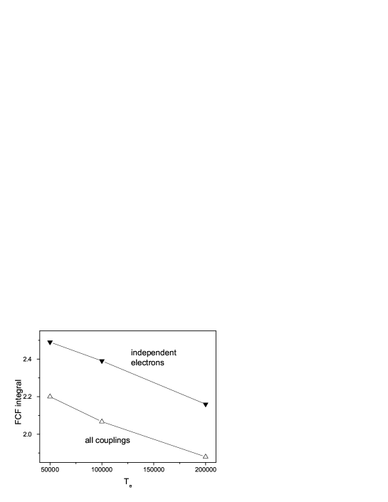
Figure 7: FCF integral versus temperature for $Z=1$. white triangles: all couplings, black triangles: independent-electrons.

It is seen that the FCF integral decreases with temperature, so evidently the dynamical effect of a decreasing correlation time dominates the increasing initial correlations. The effects of electron-impurity and electron-electron coupling leads to an approximately $15$ percent decrease in the integral at all temperatures relative to that for the independent electron model.

Finally, the $Z$ dependence of the FCF integral is demonstrated in Fig. 8. Again dynamical effects of a decreasing correlation time and anticorrelation dominate, leading to an approximately linear decrease of the integral with increasing $Z$.

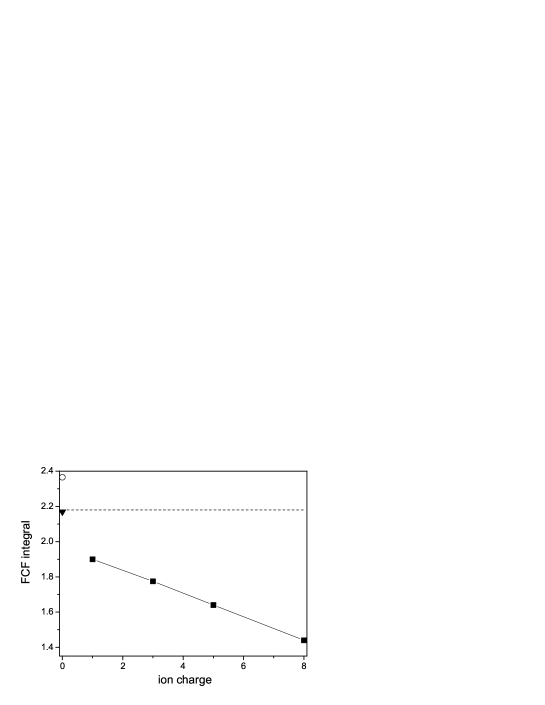
Figure 8: FCF integral versus emitter charge at $T_{e}=200000K$. Squares: all couplings; dashed: independent-electrons; triangle: all couplings with $Z=0$; circle: unscreened uncoupled electrons with $Z=0$.

Consider first the value $Z=0$ (no impurity-electron coupling). The triangle represents the results with electron-electron coupling, while the line is the independent electron model. It is seen that the use of the screened field in the latter accounts well for the relevant electron-electron coupling. This is consistent with the discussion following Fig. 3. Also shown is the independent electron model without using the screened fields (open circle). This shows clearly that electron-electron coupling is almost a 10 percent effect at $Z=0$. This is significant since the electron-electron coupling constant is quite small ($\Gamma=0.029$). For $Z=1$ the electron-emitter interaction is quite important, decreasing the integral by almost $15$ percent below the independent electron value. This coupling continues to dominate for increasing $Z$. As noted above, for $Z>0$ there is an additional importance of the electron-electron coupling in the MD which is needed to establish the correct weight for the increasing number of quasi-bound orbits.

II.2 Ion-electron two component plasma MD simulations

In this subsection MD studies of an equilibrium, charge neutral two-component plasmas (TCP) of $N$ electrons and $N/Z_{i}$ ions are reported. Charge neutrality is guaranteed by the charge concentration. Preliminary classical TCP MD simulations in this context of applications to spectroscopy have been reported elsewhere tal2 . The challenging aspect of such simulations is to move slow and fast particles at the same time. Such a study of fast and slow processes requires simulations stable over a long period of time, long enough to account for ion motion and based on a time step compatible with electron motion. This problem has been addressed mostly in the context of hydrogenic plasmas hydrogen and is extended here to higher $Z$ ions. The emitter is taken to be one of the ions of the TCP.

It is worth noting at this point the distinction between classical MD applied to the TCP, where both ions and electrons move dynamically, and “quantum MD” where the ions move classically on a self-consistent potential energy surface of the electrons Collins ; dharma . In the latter, at each time step for the ions the ground state configuration for the electrons is determined by some quantum method (e.g., density functional theory). Subsequently the forces between the ions in this electronic configuration are calculated and the ions are moved along the corresponding classical trajectory. The process is repeated at the next time step. The two classes of simulations appear complementary, with quantum MD being more appropriate for lower temperatures and semi-classical MD more appropriate at higher temperatures.

We first verify that the MD simulation properly describes the expected ion-electron screening mechanism. For this purpose the simulation of a neutral mixture of hydrogen-like carbon ions $Z=5$ in electrons has been carried out with the temperature $T_{e}=50000K$ and the electron density $N_{e}=10^{19}cm^{-3}$. As discussed following Eq. 1, a large cutoff length $\lambda$ comparable to the system size has been used in the potential to allow the periodic boundary conditions. Since the physical screening resulting from the collective effects of these “Coulomb” interactions is at a much smaller scale, this cutoff does not affect the study of that screening. A comparison of the ion-ion pair distribution function for the TCP with “Coulomb” interactions with that for a corresponding ion OCP using Debye screened interaction is made. In the OCP system there are no electrons and ion-ion Coulomb potential is screened at the Debye length phenomenologically, while such screening must be generated directly by the electrons in the TCP simulations. Figure 9 shows the rather good agreement between the two simulations, giving an indirect evidence of the effectiveness of the ion-ion dynamic screening by the electrons (also shown is the OCP without screening to quantify the effect being studied). The TCP result shows a small enhancement of the screening mechanism over that of the OCP at shorter distances. This behavior suggests that the short range ion-ion interaction could be well described using an effective ion charge $\overline{Z}<Z$. An rough estimate not shown gives $\overline{Z}\simeq 4.7$.

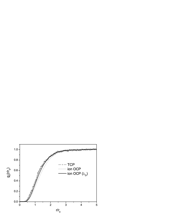
Figure 9: Pair correlation function. Solid: OCP; circles: TCP; dots: no screening.

Evidence of screening also can be demonstrated via the dynamics of the total field due to both ions and electrons at one of the ions (considered to be the emitter). MD simulation allows determination of statistical data for each particle type involved. In the electron-ion TCP two kinds of time dependencies coexist, the high frequency and the low frequency dynamics related to electron motion and ion motion, respectively. Both of them are of interest for probing or discussing the simulation procedure accuracy. For the high frequency data the electron field autocorrelation function at the ion has been calculated. This is similar to the property calculated in the subsection above for jellium, except that now it is in the presence of many other ions. Figure 10 shows a comparison of the field autocorrelation function for the field seen by a single ion in electrons (jellium) and for the TCP.

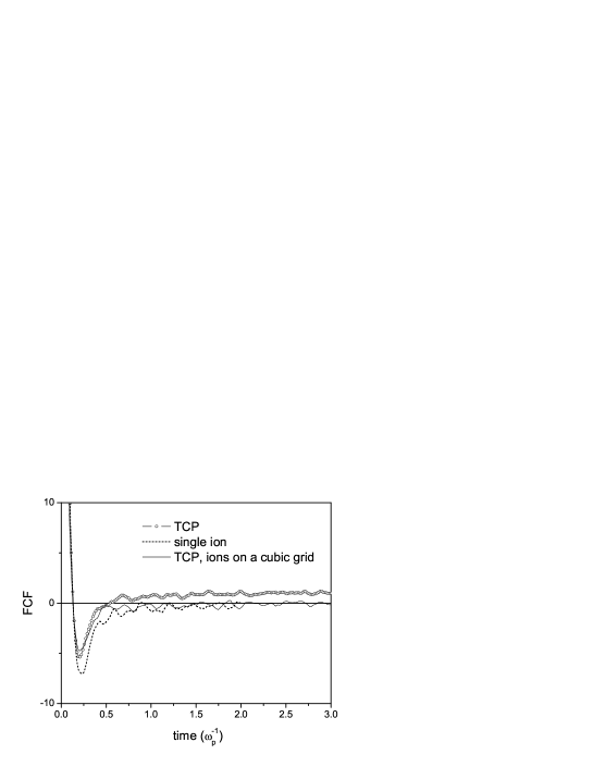
Figure 10: Electron field autocorrelation function. Dashed: impurity; circles: TCP; solid: cubic array.

Despite some noise due to insufficient sampling it can be observed that for the TCP the field correlation function does not go to $0$ as for the impurity in jellium case. The timescale used in this simulation is the inverse electron plasma frequency, compatible with the high frequency mechanisms of the electrons. On this time scale the electron FCF tends to a constant value rather than zero, denoting the occurrence of a low-frequency component in the electron field, due to its coupling to the slower ion dynamics. Contrary to the impurity ion in jellium, a given ion is no longer a center of symmetry for the average electron structure. Rather, this average electron structure is a blurred image of the random ion configuration which remains quasi-static at this time scale. This low frequency component disappears, as shown on Fig. 11, if the ions are located on the nodes of a cubic array where each ion is a center of symmetry of the infinite system. As expected, on the time scale of this low-frequency dynamics this seemingly constant value goes to $0$.

In many theoretical formulations of lineshapes, such as the fast fluctuation approximation of the next section, it is assumed that the electron electric field relaxes quickly relative to the time scale of the emission or absorption process. One consequence of the occurrence of a low-frequency component in the TCP electron field is that these approximations are no longer valid.

The FCFs generated by a one component plasma of ions interacting through a Coulomb potential 1) with a screening length $\lambda_{D}=$ Debye length, 2) with a box screening length $\lambda>\lambda_{D}$ are compared with the FCF of the low frequency field component of the ion plus electron total field on Fig. 11.

Figure 11: Total field autocorrelation function. Dots: TCP simulation; solid: ion OCP simulation; dashed: ion OCP no screening.

The good agreement of the two curves and the large discrepancy with the no screening result can be interpreted again as the proof that the screening mechanisms take place properly in the TCP molecular dynamics simulations.

III Electron-ion coupling effects on lineshape

III.1 Dipole relaxation mechanisms

Linear response methods can be applied to the dipole relaxation of a quantum emitter in a classical plasma environment griem . According to the energy involved it is postulated that the perturbation by the environment never induces transitions between the two manifolds for which the transition is considered within the characteristic time of the emission - no quenching approximation. This approximation therefore neglects emitter-bath coupling via the radiated dipole transition and any contribution of the dipole transition moment at equilibrium. As a result, the spectral profiles of dipole spontaneous-emission are given in terms of the autocorrelation function $C(t)$ of the system dipole moment $\mathbf{q}(t)$, via a Fourier transformation:

$$I(\omega) = {\rm Re}\frac{1}{\pi}\int_{0}^{\infty}dt~{}C(t)\,e^{{\rm i}\omega t}\,,$$ (3)

$$C(t) = {\rm tr}\;\{U^{*}(t)\rho\,\mathbf{q}U(t)\cdot\mathbf{q}\}$$ (4)

The trace is taken over an equilibrium Gibbs statistical ensemble $\rho$ for the total system of plasma plus emitter. The Hamiltonian is taken to be the sum of the plasma Hamiltonian (including the point monopole of the emitter) $H_{p}$, the Hamiltonian for the internal states of the emitter $H_{e}$, and their interaction due to the plasma electric field coupling to the internal emitter dipole. For simplicity here, the Doppler broadening due to emitter center of mass motion has been assumed to be statistically independent of this dipole broadening. The operator $\mathbf{q}(t)=U(t)\mathbf{q}U^{*}(t)$ obeys the Heisemberg equation

$${\rm i}\hbar\frac{d\mathbf{q}(t)}{dt}=[H_{e}-\mathbf{E}(t)\cdot\mathbf{d},\mathbf{q}(t)]$$ (5)

The second term in the commutator describes the perturbation due to the total electric field of the plasma $\mathbf{E}(t)$. Due to the no quenching approximation, $\mathbf{d}$ is restricted here to the part of the internal emitter dipole operator coupled to this field. The time dependence of $\mathbf{E}(t)$ is generated by the plasma Hamiltonian alone. This shows most directly the utility of MD simulation in addressing the most difficult part of a line broadening problem: identifying properly and completely the environment of the emitter. In the present case this is given by an electric field history. To represent an equilibrium ensemble for the environment a collection of field histories for different initial conditions is given, the Schrödinger equation solved in each case, and a simple algebraic average is performed over all such solutions to get the line profile. In practice the numerical solution to the Schrödinger equation can be straightforward or complicated depending on the electric field history. This is the case for high $Z$ radiators for which the quasi bound orbits described above can give rise to high frequency, strong fields (e.g., as in Fig. 6). The calculations require a fast integration process based on a polynomial development using the so called Euler-Rodrigues coefficients. A detailed presentation of the method applied to hydrogenic lines has been given elsewhere marco .

The existing theoretical analysis generally entails further approximations not necessary in the above MD/Schrödinger equation simulation. Due to the small electron-ion mass ratio, Stark effects resulting from slow ion and fast electron micro-fields are generally considered separately. The Stark effect due to ions is approximated by a static electric field, while electron broadening is described as a dynamical process resulting from the high frequency fluctuation of the electron electric field. The usual approach for electron broadening griem for ion emitters in plasmas is a binary collision model involving independent electrons moving on straight trajectories at constant velocity. Electron correlations are accounted for only indirectly by screening the electron-emitter potential at the Debye length. There are other theoretical models with different approximations, but for the discussion here we will primarily compare simulations for two cases: 1) the electrons are considered as free particles that do not interact with each other but perturb the ion emitters with a field obtained from the potential written in Eq. (2) with $\lambda=\lambda_{D}$; and 2) the electrons have Coulomb interactions with each other and couple to the emitter with a field obtained using Eq. (2) with $\lambda=s/2$. The latter, of course, is the correct treatment of correlations.

A more compact formulation of the problem is obtained using a Liouville operator representation fano allowing to disentangle the evolution operator from the internal emitter dipole operator $\mathbf{q}$. Liouville operators are defined according to the following relation: $L_{0}\equiv\frac{1}{{\rm i}\hbar}[H_{0},\cdot]$. In this representation the dipole correlation function can be rewritten $C(t)=Tr(\bf{q}\cdot U(t)\rho\bf{q})$. Equation 5 is replaced by the following stochastic equation for the evolution operator alone:

$$\frac{dU_{\alpha}(t)}{dt} = (L_{0}+\mathbf{D}\cdot\mathbf{E}_{\alpha}(t))U_{\alpha}(t),\quad U_{\alpha}(0)=1$$

$$\textbf{U}(t) = \{U_{\alpha}(t)\}_{av}=\frac{1}{N}\sum_{\alpha=1}^{N}U_{f_{\alpha}}(t)$$ (6)

where $\mathbf{E}_{\alpha}(t)$ is one of the electric field histories, $\mathbf{D}$ is the Liouville representation of $\mathbf{d}$ and $\mathbf{U}(t)$ denotes the solution of the stochastic equation.

A useful approximation described in Appendix A, the fast fluctuation limit, can be obtained when the characteristic time for the field correlation function is much smaller than the typical relaxation time of the physical process investigated - here the dipole lineshape . In this limit the stochastic equation reduces to:

$$\frac{d\textbf{U}(t)}{dt}=(L_{0}-\textbf{W})\textbf{U}(t)$$ (7)

where W is proportional to the field correlation function integral $\int_{0}^{\infty}\{\mathbf{E}_{\alpha}(0)\cdot\mathbf{E}_{\alpha}(t)\}_{\alpha}dt$. Thus questions regarding the effects of charge-charge coupling on the linewidth can be addressed directly from the simulation of the field autocorrelation function as described in the previous sections.

III.2 Electron broadening

The purpose of this section is to apply the EBT developed herein for discussing the occurrence of charge-charge coupling effects in electron broadening. This issue is motivated in part by recent experimental and theoretical studies performed on a series of lines emitted by ions of increasing charge 3s3p . The specificity of these lines relies on the absence of ion broadening. However, in contrast, the present study concerns lines with ion broadening so the generalization of the conclusions here to all kinds of lines would be inappropriate. Ion lines with non negligible ion broadening have been selected as they fit also the objective of studying Stark broadening in two component plasmas accounting for complete charge-charge coupling.

According to the EBT, the study of electron broadening relies first on the construction of large field sample-sets at the emitter generated by molecular dynamics. Then, the lineshape or simply the full width at half maximum (FWHM), $\gamma(Z,T_{e})$, is obtained after numerical solutions of the Schrödinger equation and its average. Due to the various characteristic times of the problem, a given field history can be split into a number of independent samples depending on the final purpose. In the present case, the dipole relaxation simulation requires samples much more longer than those necessary to obtain the field statistical properties. In addition, the study of electron broadening as a function of the emitter charge can be limited by calculation costs, since the dipole response of the emitter decreases as the inverse of the square of the emitter charge. For instance, to carry out an equivalent study with respect to the noise inherent to this kind of statistical average for emitters of net charge $Z=1$ and $Z=8$, it would be necessary to generate a field sample set and then integrate the Schrödinger equation over a time about $20$ times longer for $Z=8$ than for case $Z=1$. Accordingly, the present study is limited to cases relevant for the fast fluctuation limit (FFL) allowing a simpler theoretical representation of the line width and thereby avoiding the full integration process. It should be noted that, for a given temperature, if conditions for the FFL are fulfilled for a chosen line in the case $Z=1$ they are even more relevant for the same line in the case $Z=8$. However, the dipole autocorrelation will be calculated by complete integration of the Schrödinger equation in a few cases in order to check the FFL and for cross comparisons. In order to probe the statistical properties of the local microfield, Balmer-alpha lines for hydrogen like emitters of charge $Z=1,3,5,8$ have been chosen together with the three plasma temperatures $T=5\times 10^{4},10^{5},2\times 10^{5}K$ selected for this study. Both the dipole moments of the lower and the upper level manifolds are coupled to the perturbing field giving rise to the relaxation process and line broadening of the emitted dipole transition $n=3\rightarrow n=2$. Qualitatively, for the Balmer alpha line, the electric field perturbation induces two opposite broadening mechanisms, i.e. the line broadening increases with the covariance characteristic of the field strength while, due to some time averaging inherent to the dipole relaxation process, it decreases with an increasing fluctuation dynamics of the perturbation.

Table 1: Balmer alpha FWHM $(s^{-1})$ versus temperature for $Z=1$.

Temperature	$\gamma_{FFL}$	$\gamma_{SE}$
$5\times 10^{4}K$	$10.7\times 10^{12}$	$11.8\times 10^{12}$
$10^{5}K$	$9.88\times 10^{12}$	$10.2\times 10^{12}$
$2\times 10^{5}K$	$9.32\times 10^{12}$	$9.93\times 10^{12}$

Comparisons of the FWHM are reported in Tab. 1, where $\gamma_{FFL}$ is the fast fluctuation limit result and $\gamma_{SE}$ results from simulation i.e. from a full integration of the Schrödinger equation. The discrepancy is smaller than $10\%$ of the FWHM. In addition the exponential decay of $C(t)$ predicted by the FFL also is confirmed for the simulations (not shown).

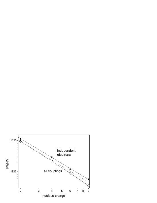
Figure 12: Balmer-alpha FWHM, $Z=1$, $T_{e}=200000$ K. Squares: independent-electrons; solid line: independent-electron linear fit; circles: charge-charge coupling; black triangle: complete integration; dots: $1/(Z+1)^{2}$ line.

For the high temperature case, these results are plotted on a log scale in Fig. 12, versus the nucleus charge, together with the corresponding independent electron calculations (free electrons moving on straight trajectories that perturb the emitter via the potential defined in Eq. 2 screened at the Debye length). The field sampling generation cost by the MD technique is quite low for noninteracting particles. Therefore, these calculations can be performed by integration of the stochastic equation with a satisfactory noise level. The FWHM calculations fit the $1/(Z+1)^{2}$ behavior even without coupling to the emitter due to the atomic physics dependence (dipole matrix elements) of the linewidth. These calculations confirm the capability of the simulation technique to provide relevant results even in the fast fluctuation limit domain. The entire discrepancy between the two results of Fig. 12 is therefore a consequence of the charge-charge coupling in the time integral of the FCF as a function of the emitter charge (i.e., the effect discussed in Fig. 8). This discrepancy increases with decreasing temperature as shown in Fig. 7.

III.3 Coupled ion-electron broadening

It has been shown in a previous section that classical two component MD simulations provide relevant results regarding charge structure and dynamics. The plasma conditions have been selected to emphasize screening mechanisms in order to demonstrate significative effects. Other results obtained for weaker coupling conditions lead to the same observations. These investigations ensure that ion plus electron field samplings are properly generated by the MD simulation for the plasma conditions of this work. Like for the EBT, field sampling is the first stage of the ion electron broadening theory (IEBT). In the second stage these fields are used for integrating the Schrödinger equation in order to synthesize lineshapes. This protocol requires a numerical cost much smaller than for the impurity case because 1) a number of samples are generated at the same time using each ion as the emitter, and 2) the integration time required for $C(t)$ is shorter when ion broadening is accounted for.

Figure 13: Helium hydrogen-like Balmer alpha line $T_{e}=50000$ K.

Two field data sets are used in order to look for evidences of ion-electron coupling mechanisms at the lineshape level. The two data-sets are built using TCP molecular dynamics techniques, 1) with all the charge-charge interactions accounted for and, 2) taking into account only the ion-ion interactions assuming a Debye screening for the ion-ion potential and free electrons moving on straight trajectories. The observed discrepancy in Fig. 13 is a decrease of $6-7\%$ in the full width at half maximum when both the ion-electron and the electron-electron coupling are accounted for.

IV Conclusion

Semi-classical models involving a quantum emitter perturbed by a stochastic classical electric field have been developed to calculate emitter dipole relaxation. On this basis charge correlation effects relevant for plasma spectroscopy have been explored. Such reference results from ideal numerical experiments are indispensable, particularly when the plasma conditions are such that the usual theoretical approximations appear questionable. The calculations reported here are for two distinct models, with and without ion-electron and electron-electron couplings. They give rise to comparisons of two sets of line broadening calculations. The observed residual discrepancies confirm that effects of charge-charge couplings on lineshapes can be non negligible.

Common electron broadening theories do not account for ion-electron couplings. The main reason is that for most of the ionic lines (normal lines) electron broadening is a small effect with respect to ion broadening. This has not motivated the development of theories accounting for the complex problem of the quantum properties of a charged emitter undergoing a perturbation resulting from the electrons around the charge. However, this interest exists for lines whose broadening is dominated by the electrons. In this work charge-charge coupling effects on ionic lines have been investigated considering electron broadening of lines with ion broadening. It is worth analyzing the main results obtained here with the impact theory for comparison. This theory is founded on the hypothesis that strong collisions do not overlap in time. Collision operators for electron broadening have been derived on this basis using either linear or parabolic electron trajectories alexiou . For the electrons attracted to the ion impurity the impact theory postulate of binary encounters is no longer correct as the close electron trajectories depend on the other close electrons via kinetic energy exchanges, particularly in the case of temporary orbiting trajectories. Accordingly it can be concluded that ion-electron couplings cannot be treated ignoring electron-electron couplings. In terms of the electric field dynamics, these couplings induce an increase of both the covariance and the field fluctuation rate when the emitter charge or the temperature increase. These effects result in a decrease of the width of the studied lines in comparison with the uncoupled case.

Both the EBT and the IEBT have been designed to account for all charge-charge couplings. They are based on the numerical integration of the Schrödinger equation over a large electric field sample set generated by molecular dynamics techniques. For the selected lines and plasma conditions the fast fluctuation limit provides a simple theoretical expression for electron broadening in terms of the time integral of the field autocorrelation function. This approximation has been checked by comparisons with a few results obtained by full integration of the Schrödinger equation. In parallel to this work MD simulations and theoretical studies of the FCF for an ion impurity in jellium have been carried out with preliminary results reported in dufty-ilya . Thus, the FCF and the fast fluctuation limit provide an efficient prediction of the linewidth for this simple impurity case. In contrast, it appears that integration of the Schrödinger equation appears easier when both ion and electron broadening occur together, using two component plasma MD simulations for the field histories. It has been shown here that such TCP simulations reliably yield the proper dynamic electron screening of the ion-ion forces.

Finally, it can be noted that the direct integration of the Schrödinger equation for lineshapes can be rather intricate and expensive. Despite the apparent difficulty of this step by step integration process, it appears robust enough to give accurate results that can be seen as ideal experiments providing reference data appropriate to discuss or benchmark other theories.

Appendix A Fast fluctuation limit

In this Appendix an outline of the fast fluctuation limit for the line profile is given. The terminology “fast fluctuation limit” used instead of the alternative “impact limit” has been preferred to avoid confusing it with the impact theories. The later relies on the calculation of an average binary collision - the collision operator. The impact theories generally postulate non overlapping strong collisions, which is not a limitation of the fast fluctuation limit obtained here.

A.1 Characteristic time scales

Three characteristic time scales have to be considered. First, the typical correlation time of the perturbing field $\mathbf{E}(t)$, and in consequence, the characteristic time of $L(t)$. This time scale is ruled by the kinetics of the charged particles in the plasma. Its order of magnitude is

$$\tau_{c}\simeq\frac{r_{0}}{v_{0}}$$ (8)

where $r_{0}$ denotes typical inter-particle distance, $v_{0}$ mean thermal velocity.

A second time scale is fixed by the correlations of the dipole-moment $\mathbf{q}(t)$. The spectral width is determined by this lifetime, $\tau_{d}$, which is, in a way, the “unknown variable” of the problem.

Finally, a time scale is fixed by characteristic values of $L$ :

$$\frac{1}{\tau_{H}}\simeq L\simeq\frac{1}{\hbar}eE_{0}\frac{n^{2}a_{0}}{Z}$$ (9)

$a_{0}$ is the Böhr radius, $n$ the principal quantum number of the upper group of states. Evolution of the dipole moment $\mathbf{q}(t)$ would be fixed by this frequency scale if the perturbing electric field were stationary.

The relationship between $\tau_{H}$ and $\tau_{c}$ will determine the relevant physical phenomenon in spectral line broadening. $\tau_{c}\geq\tau_{H}$ is the condition for “quasistatic” broadening which is a close limit for ion broadening. Both shape and width of the spectral line are fixed by the statistical distribution of the perturbing fields, then $\tau_{d}\sim\tau_{H}$.

If $\tau_{c}\ll\tau_{H}$ the evolution of the dipole moment $\mathbf{q}(t)$ is much slower than the evolution of the perturbing fields. This condition fits the electron broadening mechanisms. In this case, perturbations are less efficient, since the emitter responds to a time average of the electric field smaller than its statistical typical value. It is the fast fluctuation regime. In the next section it will be seen that in this regime the dipole autocorrelation fits well a decreasing exponential whose lifetime $\tau_{d}\gg\tau_{H}>\tau_{c}$, is determined by the autocorrelation function of the perturbing field. It should be noted that in the present study the ratio $\tau_{c}/\tau_{d}$ varies from a few hundreds to a few thousands. Such a large ratio guarantees that the FFL is totally relevant as the discrepancy of the dipole autocorrelation function to an exponential (or equivalently the discrepancy of the lineshape to a Lorentzian) is non significant.

A.2 Fast fluctuation limit

The dipole correlation function of the text can be rewritten as

$$C(t)={\rm tr}\;\{\,{\bf q}(t)\cdot{\bf q}\rho\,\}={\rm tr}_{e}\;\left(\,{\rm tr}_{p}\;\{\,e^{Lt}\rho{\bf q}\,\}\right)\cdot{\bf q}$$ (10)

The trace has been separated into that for the emitter and plasma subspaces, stationarity of the Gibbs ensemble under the dynamics has been used, and the Liouville operator $L$ generating the dynamics has been introduced. It is the sum of the Liouville operator for the emitter in the relative coordinate system, $L_{e}$, the Liouville operator for the plasma including the center of mass (point monopole) of the emitter, $L_{p}$, and the coupling between the internal emitter states and the plasma, $L_{i}$

$$L=L_{e}+L_{p}+L_{i}$$ (11)

Define the interaction representation generator by

$$e^{Lt}=e^{\left(L_{e}+L_{p}\right)t}U(t)=e^{\left(L_{e}+L_{p}\right)t}\;T\;\exp\int_{0}^{t}dt^{\prime}L_{i}(t^{\prime}).$$ (12)

Here $T$ is the time ordering operator with largest times to the left. Then

$$C(t)\equiv{\rm tr}_{e}\;\left(\,e^{(L_{e}+L_{p})t}\,e^{\widehat{O}(t)}\,f_{e}{\bf q}\,\right)\cdot{\bf q}$$ (13)

where $\widehat{O}(t)$ is the average generator for the interaction dynamics in the atomic subspace

$$e^{\widehat{O}(t)}={\rm tr}_{p}\;T\;\exp\int_{0}^{t}dt^{\prime}L_{i}(t^{\prime})\rho f_{e}^{-1}=\langle T\;\exp\int_{0}^{t}dt^{\prime}L_{i}(t^{\prime})\rangle_{p},\hskip 21.68121ptf_{e}={\rm tr}_{p}\;\rho$$ (14)

The leading terms in a cumulant expansion of this average are

$$\widehat{O}(t)=\widehat{O}^{(1)}(t)+\widehat{O}^{(2)}(t)+..$$ (15)

with

$$\widehat{O}^{(1)}(t)=\int_{0}^{t}dt^{\prime}\langle L_{i}(t^{\prime})\rangle_{p}$$ (16)

$$\widehat{O}^{(2)}(t)=\int_{0}^{t}dt^{\prime}\int_{0}^{t^{\prime}}dt^{\prime\prime}\;\langle\widetilde{L}_{i}(t^{\prime})\widetilde{L}_{i}(t^{\prime\prime})\rangle_{p}=t\,\int_{0}^{t}dt^{\prime}\left(1-\frac{t^{\prime}}{t}\right)\langle\widetilde{L}_{i}(t)\widetilde{L}_{i}(t^{\prime})\rangle_{p}$$ (17)

where

$$\widetilde{L}_{i}(t^{\prime})=L_{i}(t^{\prime})-{\rm tr}_{p}\;L_{i}(t^{\prime})\rho f_{e}^{-1}$$ (18)

The fast fluctuation limit corresponds to the case where the perturber dynamics varies rapidly on the time scale of the dipole correlation function $C(t).$ Since the average is performed only over the plasma degrees of freedom this time scale is controlled by the perturbers. Then the fluctuation in Eq. (17) decays to zero for $t^{\prime}=\tau\ll t$ and the factor $t^{\prime}/t$ in the integrand can be neglected

$$\widehat{O}^{(2)}(t)\rightarrow t\int_{0}^{t}dt^{\prime}\langle\widetilde{L}_{i}(t)\widetilde{L}_{i}(t^{\prime})\rangle_{p}$$ (19)

For similar reasons, higher order terms in the cumulant expansion are expected to be of higher order in $\tau/t$ and therefore negligible.

Further simplifications occur with additional assumptions. If the interaction is only through a coupling of the emitter dipole to the plasma field then $L_{i}=-{\bf E}\cdot{\bf D}$. Also, if the emitter-plasma interactions are neglected in $\rho f_{e}^{-1}$ then

$$\rho f_{e}^{-1}\rightarrow\rho_{p}$$ (20)

and the fluctuations become

$$\langle L_{i}(t)\rangle_{p} \rightarrow 0,$$

$$\langle\widetilde{L}_{i}(t)\widetilde{L}_{i}(t^{\prime})\rangle_{p} \rightarrow \frac{1}{3}\Gamma(t-t^{\prime}){\bf D}(t){\bf\cdot D}(t^{\prime})$$ (21)

where $\Gamma(t)$ is the electric field autocorrelation function for the plasma alone

$$\Gamma(t)=\langle{\bf E}(t)\cdot{\bf E(0)}\rangle_{p}$$ (22)

and the dipole operator in ${\bf D}(t)$ has a time dependence due to the emitter alone. Finally, in the case of an emitter with upper and lower degenerate manifolds such as the Balmer alpha line without fine structure this time dependence of the dipole operators can be neglected as well. The result quoted in the text is then obtained

$$C(t)\equiv{\rm tr}_{a}\;\left(e^{L_{e}t}e^{t\left(\int_{0}^{\infty}dt^{\prime}\,\Gamma(t^{\prime})\,{\bf D\cdot D}\right)}f_{e}{\bf q}\right)\cdot{\bf q}$$ (23)

References

- (1) H.R. Griem, A.C. Kolb and K.Y. Shen, Phys. Rev. 116,4(1959); H.R. Griem, A.C. Kolb and K.Y. Shen, Astrophys. J. 135,272(1962)
- (2) D. Voslamber, Z. Naturforsch, 24a,1458(1969); E.W. Smith, J. Cooper and C.R. Vidal, Phys. Rev, 185,140(1969)
- (3) J.P. Hansen, I.R. McDonald and E.L. Pollock, Phys. Rev. A 11,1025(1975)
- (4) B. Talin, A. Calisti and J. W. Dufty, Phys. Rev. E 65, 056406(2002).
- (5) B. Talin, E, Dufour, A. Calisti, M. A. Gigosos, M. A. González, T. del Río Gaztelurrutia and J. W. Dufty, J.Phys. A 36, 6049(2003); E. Dufour, A. Calisti, B. Talin, M. A. Gigosos, M. A. González and J.W. Dufty, JQSRT, 81,125(2003)
- (6) R. Stamm, B. Talin, E.L. Pollock and C.A. Iglesias, Phys. Rev. A 34,4144(1986)
- (7) H. Minoo, M.-M. Gombert, and C. Deutsch, Phys. Rev. A 23, 924 (1981).
- (8) J. W. Dufty, I. Pogorelov, A. Calisti and B. Talin, J.Phys A 36, 6067(2003); J. W. Dufty, I. Pogorelov, A. Calisti and B. Talin, ”Electron Dynamics at a Positive Ion”, submitted to Phys. Rev. E.
- (9) Yu. V. Ralchenko, H. R. Griem and I. Bray, JQSRT 81, 371(2003); H. Hegazy, S. Seidel, Th. Wrubel and H.-J. Kunze, JQSRT 81,221(2003)
- (10) F. J. Rogers, J. Chem. Phys. 73, 6272 (1980); Phys. Rev. A 29, 868 (1984).
- (11) J.P. Hansen and I. R. MacDonald, Phys. Rev. A23,2041 (1981); G. E. Norman, A. A. Valuev, and I. A. Valuev, J. Phys. IV France 10, Pr5-255 (2000); T. Pschiwul and G. Zwicknagel, Contrib. Plasma Phys. 41, 271 (2001).
- (12) L. Collins, I. Kwon, J. Kress, N. Troullier, and D. Lynch, Phys. Rev. E 52, 6202(1995).
- (13) C. Dharma-Wardana in Strongly Coupled Plasmas, 275, H. de Witt, and F. Rogers editors (NATO ASI Series, Plenum, NY, 1987).
- (14) H. R. Griem, Spectral line broadening by plasmas. New York Academic press 1974.
- (15) M. A. Gigosos, J. Fraile, and F. Torres, Phys Rev A 31, 3509(1985); M. A. Gigosos and V. Cardeñoso, J. Phys B 20, 6005(1987); M. Gigosos and V. Cardeñoso, J. Phys B 29, 4795(1996).
- (16) U. Fano, Phys. Rev. 131, 259(1963)
- (17) M. Lewis, Phys. Rev. 121, 501 (1964); C. Cohen-Tannoudji, Aux Frontières de la Spectroscopie Laser, Vol. 1, North-Holland Publishing Company 1975)
- (18) S. Alexiou, Phys. Rev. A49, 106(1994); S.Alexiou and Y. Maron, JQSRT 53,109 (1995)