Nonlinear Whistlerons

Abstract

Recently, observations from laboratory experiments have revealed amplitude modulation of whistlers by low-frequency perturbations. We here present theoretical and simulation studies of amplitude modulated whistler solitary waves (whistlerons) and their interaction with background low-frequency density perturbations created by the whistler ponderomotive force. We derive a nonlinear a nonlinear Schrödinger equation which governs the evolution of whistlers in the presence of finite-amplitude density perturbations, and a set of equations for arbitrary large amplitude density perturbations in the presence of the whistler ponderomotive force. The governing equations studied analytically in the small amplitude limit, and are solved numerically to show the existence of large scale density perturbations that are self-consistently created by localized whistlerons. Our numerical results are in good agreement with recent experimental results where the the formation of modulated whistlers and solitary whister waves were formed.

I Introduction

Almost three decades ago, Stenzel r1 experimentally demonstrated the creation of a magnetic field-aligned density cavities by the ponderomotive force of localized electron whistlers. Observations from a recent laboratory experiment r2 exhibit the creation of modulated whistler wavepackets due to nonlinear effects. Furthermore, instruments on board the CLUSTER spacecraft have been observing broadband intense electromagnetic waves, correlated density fluctuations and solitary waves near the Earth’s plasmapause, magnetopause and foreshock r3 , revealing signatures of whistler turbulence in the presence of density depletions and enhancements. The Freja satellite r4 also observed the formation of envelope whistler solitary waves correlated with density cavities in the plasma.

A theoretical investigation has in the past predicted the self-channeling of electron whistlers and the creation of a localized density hump r5 . Taking into account the spatio-temporal dependent whistler ponderomotive force r6 ; r7 , investigations of the modulation and filamentation of finite amplitude whistlers interacting with magnetosonic waves r8 ; r9 ; r10 and ion-acoustic perturbations r11 ; r12 have been carried out.

In this article, we investigate nonlinearly interacting electron whistlers and arbitrary large amplitude ion-acoustic perturbations, by using computer simulations, and we find analytical expressions for whistlerons in the low-amplitude limit Eliasson ; Kourakis .

II Derivation of the governing equations

Let us consider the propagation of nonlinearly coupled whistlers and ion-acoustic perturbations in a fully ionized electron-ion plasma in a uniform external magnetic field $\widehat{\bf z}B_{0}$, where $\widehat{\bf z}$ is the unit vector along the $z$ direction and $B_{0}$ is the magnitude of the magnetic field strength. We consider the propagation of right-hand circularly polarized modulated whistlers of the form

$${\bf E}=\frac{1}{2}E(z,t)(\widehat{\bf{x}}+i\widehat{\bf{y}})\exp[i(k_{0}z-\omega_{0}t)]+\mbox{c.c},$$ (1)

where $E(z,t)$ is the slowly varying envelope of the whistler electric field, and $\widehat{\bf x}$ and $\widehat{\bf y}$ are the unit vectors along the $x$ and $y$ axes, respectively, and c.c. stands for the complex conjugate. The whistler frequency $\omega_{0}$ $(\gg\sqrt{\omega_{ce}\omega_{ci}})$, and the wavenumber $k_{0}$ are related by the cold plasma dispersion relation

$$\omega_{0}=\frac{k_{0}^{2}c^{2}\omega_{ce}}{\omega_{pe,0}^{2}+k_{0}^{2}c^{2}},$$ (2)

where $c$ is the speed of light in vacuum, $\omega_{ce}=eB_{0}/m_{e}c$ ($\omega_{ci}=eB_{0}/m_{i}c$) is the electron (ion) gyrofrequency, $\omega_{pe,0}=(4\pi n_{0}e^{2}/m_{e})^{1/2}$ is the electron plasma frequency, $e$ is the magnitude of the electron charge, $m_{e}$ $(m_{i})$ is the electron mass, and $n_{0}$ is the unperturbed background electron number density.

The dynamics of modulated whistler wavepacket in the presence of electron density perturbations associated with low-frequency ion-acoustic fluctuations and of the nonlinear frequency-shift caused by the magnetic field-aligned free streaming of electrons (with the flow speed $v_{ez}$), is governed by the nonlinear Schrödinger equation r12

$$i(\partial_{t}+v_{g}\partial_{z})E+\frac{v_{g}^{\prime}}{2}\partial^{2}_{zz}E+(\omega_{0}-\omega)E=0,$$ (3)

where

$$\omega=\frac{k_{0}^{2}c^{2}\omega_{ce}}{\omega_{pe}^{2}+k_{0}^{2}c^{2}}+k_{0}v_{ez},$$ (4)

and $\omega_{pe}^{2}=\omega_{pe,0}^{2}n_{e}/n_{0}$ is the local plasma frequency including the electron density $n_{e}$ of the plasma slow motion. The group velocity and the group dispersion of whistlers are

$$v_{g}=\frac{\partial\omega_{0}}{\partial k_{0}}=2\left(1-\frac{\omega_{0}}{\omega_{ce}}\right)\frac{\omega_{0}}{k_{0}}$$ (5)

and

$$v_{g}^{\prime}=\frac{\partial^{2}\omega_{0}}{\partial k_{0}^{2}}=2\left(1-\frac{\omega_{0}}{\omega_{ce}}\right)\left(1-4\frac{\omega_{0}}{\omega_{ce}}\right)\frac{\omega_{0}}{k_{0}^{2}},$$ (6)

respectively.

The equations for the ion motion involved in the low-frequency (in comparison with the whistler wave frequency) ion-acoustic perturbations are

$$\partial_{t}n_{i}+\partial_{z}(n_{i}v_{iz})=0$$ (7)

and

$$\partial_{t}v_{iz}+\frac{1}{2}\partial_{z}v_{iz}^{2}=-\frac{e}{m_{i}}\partial_{z}\phi-\frac{1}{m_{i}n_{i}}\partial_{z}p_{i},$$ (8)

where, for an adiabatic compression in one space dimension, the ion pressure is given by $p_{i}=p_{i,0}(n_{i}/n_{0})^{3}$. Here, the unperturbed ion pressure is denoted by $p_{i,0}=n_{0}T_{i}$, where $T_{i}$ is the ion temperature.

The electron dynamics in the plasma slow motion is governed by the continuity and momentum equations, viz.

$$\partial_{t}n_{e}+\partial_{z}(n_{e}v_{ez})=0$$ (9)

and

$$0=\frac{e}{T_{e}}\partial_{z}\phi-\partial_{z}\mathrm{ln}\left(\frac{n_{e}}{n_{0}}\right)+F,$$ (10)

where $T_{e}$ is the electron temperature, $\phi$ is the ambipolar potential, and the low-frequency ponderomotive force of electron whistlers is

$$F=\frac{\omega_{pe,0}^{2}}{\omega_{0}(\omega_{ce}-\omega_{0})}\left(\partial_{z}+\frac{2}{v_{g}}\partial_{t}\right)\frac{|E|^{2}}{4\pi n_{0}T_{e}}.$$ (11)

The system of equations is closed by means of quasi–neutrality

$$n_{i}=n_{e}\equiv n,$$ (12)

which is justified if $\omega_{0}<\omega_{ce}$ is fulfilled with some margin. The continuity equations for the electrons and ions give $v_{iz}=v_{ez}\equiv v_{z}$, so that

$$\partial_{t}n+\partial_{z}(nv_{z})=0.$$ (13)

Eliminating $\partial_{z}\phi$ from the governing equations for low- frequency density perturbations, we have

$$\partial_{t}v_{z}+\frac{1}{2}\partial_{z}v_{z}^{2}=-\frac{T_{e}}{m_{i}}\left[\partial_{z}\mathrm{ln}\left(\frac{n}{n_{0}}\right)-F\right]-\frac{1}{m_{i}n}\partial_{z}p_{i}.$$ (14)

The nonlinear Schrödinger equation for the whistler electric field together with the low-frequency equations form a closed set for our purposes.

II.1 Dimensionless variables

In order to investigate numerically the interaction between whistlers and large amplitude ion-acoustic perturbations, it is convenient to normalize the governing equations into dimensionless units, so that relevant parameters can be chosen. We introduce the dimensionless variables $\xi=\omega_{pi,0}z/C_{s}$, where the sound speed is $C_{s}=[(T_{e}+3T_{i})/m_{i}]^{1/2}$, $\tau=\omega_{pi,0}t$, $N=n/n_{0}$, $u=v_{z}/C_{s}$ and ${\cal E}=E/\sqrt{4\pi n_{0}(T_{e}+3T_{i})}$; the only free dimensionless parameters of the system are $\Omega_{c}=\omega_{ce}/\omega_{pi,0}$, $\kappa=k_{0}c/\omega_{pe,0}$, $\eta=T_{i}/T_{e}$ and $V_{g}=v_{g}/C_{s}$. The normalized system of equations are of the form

$$\partial_{\tau}N=-\partial_{\xi}(Nu),$$ (15)

$$\begin{split}&\partial_{\tau}\left(u-\frac{2\alpha}{V_{g}}|{\cal E}|^{2}\right)\\ &=\partial_{\xi}\left[-\frac{u^{2}}{2}-\frac{\mathrm{ln}N+1.5\eta N^{2}}{1+3\eta}+\alpha|{\cal E}|^{2}\right],\end{split}$$ (16)

and

$$\begin{split}&\partial_{\tau}{\cal E}=-V_{g}\partial_{\xi}{\cal E}+i\bigg{[}P\partial^{2}_{\xi\xi}{\cal E}\\ &+\left(\frac{1}{1+\kappa^{2}}-\frac{1}{N+\kappa^{2}}-\frac{2}{(1+\kappa^{2})^{2}}\frac{u}{V_{g}}\right)\Omega_{c}\kappa^{2}{\cal E}\bigg{]},\end{split}$$ (17)

where the constants are $\alpha=(1+\kappa^{2})^{2}\omega_{pe,0}^{2}/\omega_{ce}^{2}\kappa^{2}$ and $P=(1+\kappa^{2})(1-3\kappa^{2})V_{g}^{2}/4\kappa^{2}\Omega_{c}$. The sign of the coefficient $P$, multiplying the dispersive term in Eq. (3), depends on $\kappa$: When $\kappa<1/\sqrt{3}$, $P$ is positive and for $\kappa<1/\sqrt{3}$ we see that $P$ is negative.

III Small-amplitude solitary waves

In the small-amplitude limit, viz. $N=1+N_{1}$, $u=u_{1}$, where $N_{1}$, $u_{1}\ll 1$, Eqs. (1)–(3) yield

$$\partial_{\tau}N_{1}=-\partial_{\xi}u_{1},$$ (18)

$$\partial_{\tau}\left(u_{1}-\frac{2\alpha}{V_{g}}|{\cal E}|^{2}\right)=\partial_{\xi}\left(-N_{1}+\alpha|{\cal E}|^{2}\right),$$ (19)

and

$$\begin{split}&\partial_{\tau}{\cal E}=-V_{g}\partial_{\xi}{\cal E}\\ &+i\left[P\partial^{2}_{\xi\xi}{\cal E}+\left(N_{1}-\frac{u}{V_{g}}\right)\frac{\Omega_{c}\kappa^{2}{\cal E}}{(1+\kappa^{2})^{2}}\right],\end{split}$$ (20)

where the only nonlinearity kept is the ponderomotive force terms involving $|{\cal E}|^{2}$. It is important to remember that our nonlinear Schrödinger equation for the whistler field is based on a Taylor expansion of the dispersion relation for whistler waves around a wavenumber $k_{0}$. Thus, this model is only accurate for wave envelopes moving with speeds close to the group speed $V_{g}$, and other speeds of the wave envelopes may give unphysical results. Here, we look for whistler envelope solitary waves moving with the group speed $V_{g}$, so that $N_{1}$ and $u_{1}$ depends only on $\chi=\xi-V_{g}\tau$, while the electric field envelope is assumed to be of the form ${\cal E}=W(\chi)\exp(i\Omega\tau-ik\xi)$, where $W$ is a real-valued function of one argument. Using the boundary conditions $N_{1}=0$, $u_{1}=0$ and $W=0$ at $|\xi|=\infty$, we have $k=0$, $N_{1}=-W^{2}\alpha/(1-V_{g}^{2})$ and $u_{1}=V_{g}N_{1}$. We here note that subsonic ($V_{g}<1$) solitary waves are characterized by a density cavity while supersonic ($V_{g}>1$) envelope solitary waves are characterized by a density hump. The system of equations (4) to (6) is then reduced to the cubic Schrödinger equation

$$P\partial^{2}_{\chi\chi}W+QW^{3}-\Omega W=0,$$ (21)

where $Q=\alpha\Omega_{c}\kappa^{2}/(1+\kappa^{2})(1-V_{g}^{2})$. Localized solutions of Eq. (7) only exist if the product $PQ$ is positive. We note that $P>0$ ($P<0$) when the whistler frequency $\omega_{0}<\omega_{ce}/4$ ($\omega_{0}>\omega_{ce}/4$), and that $Q<0$ ($Q>0$) when $|V_{g}|<1$ ($|V_{g}|>1$), so in the frequency band where $\omega_{0}<\omega_{ce}/4$, only subsonic solitary waves, characterized by a localized density cavity can exist, while in the frequency band $\omega_{0}>\omega_{ce}/4$, only supersonic solitary waves characterized by a localized density hump exist. Equation (7) has exact solitary wave solutions of the form

$$W=\left(\frac{2\Omega}{Q}\right)^{1/2}\mathrm{sech}\left[\left(\frac{\Omega}{P}\right)^{1/2}(\xi-V_{g}\tau-\xi_{0})\right],$$ (22)

where $V_{g}$ and $\Omega$ and the displacement $\xi_{0}$ are the three free parameters for a given set of physical plasma parameters. Finally, we recall that the dispersion relation for the electron whistlers used here is valid if $\omega_{0}>\sqrt{\omega_{ce}\omega_{ci}}$. For subsonic whistlers having the group speed $v_{g}=C_{s}V_{g}$ (where $V_{g}<1$), where $v_{g}\approx 2\omega_{0}/k_{0}$ and $\omega_{0}\approx k_{0}^{2}c^{2}\omega_{ce}/\omega_{pe,0}^{2}$, we have $ck_{0}/\omega_{pe,0}=(C_{s}/c)(\omega_{pe,0}/\omega_{ce})V_{g}/2>(m_{e}/m_{i})^{1/4}$.

IV Numerical results

We have investigated the properties of modulated whistler wave packets by solving numerically Eqs. (1)–(3). We have here chosen parameters from a recent experiment, where the formation of localized whistler envelopes have been observed r2 . In the experiment, one has $n_{0}=1.2\times 10^{12}\,\mathrm{cm}^{-3}$ and $B_{0}=100$ G, so that $\omega_{pe,0}=6.7\times 10^{10}\,\mathrm{s}^{-1}$ and $\omega_{ce}=1.76\times 10^{9}\,\mathrm{s}^{-1}$, respectively. Hence, $\omega_{ce}/\omega_{pe,0}=0.026$. The frequency of the whistler wave is $\omega_{0}=2\pi\times 160\times 10^{6}\,\mathrm{s}^{-1}=1.0\times 10^{9}\,s^{-1}$, so that $\omega_{0}/\omega_{ce}\approx 0.57>0.25$. Thus, the whistlers have negative group dispersion. From the dispersion relation of whistlers, we have $\kappa\approx 1.15$, which gives $k_{0}\approx 257\,\mathrm{m}^{-1}$. The latter corresponds to whistlers with a wavelength of 2.4 cm. Furthermore, the whistler group velocity is $v_{g}=3.36\times 10^{6}$ m/s. The argon ion-electron plasma ($m_{i}/m_{e}=73400$) had the temperatures of $T_{e}=10$ eV and $T_{i}=0.5$ eV, giving the sound speed $5.25\times 10^{3}\,\mathrm{m/s}$, and the normalized group velocity $V_{g}=v_{g}/C_{s}=640$.

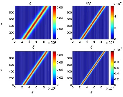
Figure 1: Simulations of solitary whistler waves, with its associated electric field envelope $|{\cal E}|$ (left panels) and density perturbation $\delta N=N-1$ (right panels). Parameters are: $V_{g}=640$, $\kappa=1.15$, $\Omega_{c}=\omega_{ce}/\omega_{pi,0}=7.05$, $m_{i}/m_{e}=73400$ (argon ions) and $\eta=0.05$. For the initial condition, we used the small-amplitude solitary wave solution ${\cal E}=W=(2\Omega/Q)^{1/2}\mathrm{sech}[(\Omega/P)^{1/2}(\xi-2.5\times 10^{5})]$, with $Q=-0.025$ and $P=-7.57\times 10^{4}$ for the given parameters, and $\Omega=-0.5\times 10^{-4}$ (upper panels) and $\Omega=-1\times 10^{-4}$ (lower panels). For the density and velocity, we used $N=1+N_{1}$ and $u=u_{1}$, where $N_{1}=-W^{2}\alpha/(1-V_{g}^{2})$ and $u_{1}=V_{g}N_{1}$.

In Fig. 1, we have illustrated localized whistler envelope solitons, in which the electric field envelope (left panels) is accompanied with a density hump (right panels). We notice that the density hump is relatively small, due to the large (in comparison with the acoustic speed) group velocity of the whistler waves.

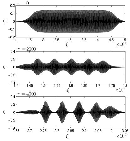
Figure 2: The electric field as a function of normalized space $\xi$ at the times $\tau=0$ (upper panel), $\tau=2000$ (middle panel) and $\tau=4000$ (lower panel). The initial condition was a pulse on the form ${\cal E}=0.07\{1-\tanh[5\cos(\pi\xi/3.1\times 10^{5})]\}$, while the density was perturbed as $N=1+0.01\cos(20\pi\xi/6.2\times 10^{5})$. Parameters are: $V_{g}=640$, $\kappa=1.15$, $\Omega_{c}=\omega_{ce}/\omega_{pi,0}=7.05$, $m_{i}/m_{e}=73400$, $\eta=0.05$. The (scaled by $C_{s}/\omega_{pi,0}$) wavelength of the high-frequency wave is $\lambda_{0}=1.16\times 10^{3}$, corresponding to $\sim 2.5$ cm in dimensional units. The envelope $\pm|{\cal E}|$ was plotted together with the real part of the wave ${\cal E}\exp(iK_{0}\xi)$, where $K_{0}=k_{0}C_{s}/\omega_{pi}=2\kappa^{2}\Omega_{c}/(1+\kappa^{2})^{2}V_{g}$. We see the formation of separate wavepackets of the modulated high-frequency wave.

In Fig. 2, we can see the development of a large-amplitude whistler pulse, which has been launched in a plasma perturbed by ion-acoustic waves, with a density modulation of one percent (see the caption of Fig. 2). This simulates, to some extent, the experiment by Kostrov et al., where the density and magnetic field were perturbed by a low-frequency conical refraction wave, giving rise to a modulation of the electron whistlers. Here, as in the experiment, we observe that a modulated electron whistler pulse (middle panel of Fig. 2) develops into isolated solitary electron whistler waves (lower panel). We note that the wavelength of the whistlers is $\approx 2.5$ cm, while the typical width of a solitary pulse is $\Delta\xi\approx 3\times 10^{4}$ in the scaled length units, corresponding to $\approx 64$ cm, so that each solitary wave train contains 25 wavelengths of the high-frequency whistlers. In one experiment, illustrated in the lower panel of Fig 4 in Ref. r2 , one finds that the width of the solitary whistler pulse in time is $0.2\,\mathrm{\mu s}$, which with the group speed $v_{g}=3.36\times 10^{6}$ m/s gives the width $\sim 60$ cm in space of the solitary wave packets, in good agreement with our numerical results. From the relation $N_{1}=-W^{2}\alpha/(1-V_{g}^{2})$ valid for solitary whistlers in the small-amplitude limit, and with the amplitude of $W=|{\cal E}|$ approximately $0.3$ seen in the lower panel of Fig. 2, we can estimate the relative amplitude of the density hump associated with the solitary waves to be of the order $10^{-3}$, i.e. much smaller than the modulation $\sim 10^{-2}$ due to the ion-acoustic waves excited in the initial condition.

Next, we study the properties of subsonic whistler envelope solitary pulses which have the normalized group speed $V_{g}=0.5$. Here, the restrictive condition $ck_{0}/\omega_{pe,0}=(C_{s}/c)(\omega_{pe,0}/\omega_{ce})V_{g}/2>(m_{e}/m_{i})^{1/4}$ requires somewhat higher values of the plasma temperature and $\omega_{pe,0}/\omega_{ce}$ for their existence. With $m_{i}/m_{e}=30000$, we have $(m_{e}/m_{e})^{1/4}\approx 0.1$. We take $\kappa=ck_{0}/\omega_{pe,0}=0.2$, $C_{s}=10^{5}$ m/s (corresponding to $T_{e}\sim 1400$ eV) $\eta=0.1$, and $\omega_{pe,0}/\omega_{ce}=2400$. Thus, $\Omega_{c}=0.072$ and $\omega_{0}/\omega_{ce}\approx 0.039$. For these values of the parameters, there exist solitary whistler pulse solutions, which we have displayed in Fig. 3.

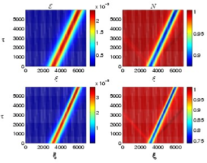
Figure 3: Simulations of solitary whistler waves, with its associated electric field envelope $|{\cal E}|$ (left panels) and density $N$ (right panels). Parameters are: $V_{g}=0.5$, $\kappa=0.2$, $\Omega_{c}=\omega_{ce}/\omega_{pi,0}=0.072$, $m_{i}/m_{e}=30000$, $\eta=0.1$. For the initial condition, we used the small-amplitude solitary wave solution ${\cal E}=W=(2\Omega/Q)^{1/2}\mathrm{sech}[(\Omega/P)^{1/2}(\xi-3000)]$, with $Q=5.5\times 10^{5}$ and $P=10.8$ for the given parameters, and $\Omega=1.5\times 10^{-4}$ (upper panels) and $\Omega=3\times 10^{-4}$ (lower panels). For the density and velocity, we used $N=1+N_{1}$ and $u=u_{1}$, where $N_{1}=-W^{2}\alpha/(1-V_{g}^{2})$ and $u_{1}=V_{g}N_{1}$.

We have used the exact solution in the small-amplitude limit as an initial condition for the simulation of the full system of equations (1)–(3). The bell-shaped whistler electric field envelope is accompanied with a large-amplitude plasma density cavity.

V Discussion

We have presented theoretical and simulation studies of nonlinearly interacting electron whistlers and arbitrary large amplitude ion-acoustic perturbations in a magnetized plasma. For this purpose, we have derived a set of equations which describe the spatio-temporal evolution of a modulated whistler packet in the present of slowly varying plasma density perturbations. The ponderomotive force of the latter, in turn, modifies the local plasma density in a self-consistent manner. Numerical solutions of the governing nonlinear equations reveal that subsonic envelope whistler solitons are characterized by a bell- shaped whistler electric fields that are trapped in self-created density cavity. This happens when the whistler wave frequency is smaller than $\omega_{ce}/4$, where the waves have positive group dispersion. When the whistler wave frequency is larger than $\omega_{ce}/4$, one encounters negative group dispersive whistlers and the supersonic whistler envelope solitons are characterized by a bell-shaped whistler electric fields which create a density hump. Modulated whistler wavepackets have indeed been observed in a laboratory experiment r2 as well as near the plasmapause r3 and in the auroral zone r4 . Our results are in excellent agreement with the experimental results r2 , while we think that a multi-dimensional study, including channelling of whistler waves in density ducts, is required to interpret the observations by Cluster and Freja satellites.

References

• (1) Stenzel R. L., Filamentation of large amplitude whistler waves, Geophys. Res. Lett.3, 61-64 (1976).
• (2) Kostrov A. V., Gushchin, M. E., Korobkov, S. V., and Strikovskii A. V., Parametric Transformation of the amplitude and frequency of a whistler wave in a magnetoactive plasma, JETP Lett. 78, 538-541 (2003).
• (3) Moullard O., Masson A., Laasko H. et al., Density modulated whistler mode emissions observed near the plasmapause, Geophys. Res. Lett.29, doi:10.1029/2002GL015101 (2002).
• (4) Huang G. L., Wang D. Y., and Song, Q. W., Whistler waves in Freja observations, J. Geophys. Res. 109, A02307, doi:10.1029/2003JA011137 (2004).
• (5) Weibel E. S., Self-channeling of whistler waves, Phys. Lett. 61A, 37-39 (1977).
• (6) Washimi H. and Karpman V. I., The ponderomotive force of a high-frequency electromagnetic field in a dispersive medium, Soviet Phys. JETP 44, 528-531 (1976).
• (7) Tskhakaya D. D. , On the ‘non-stationary’ ponderomotive force of a HF field in a plasma, J. Plasma Phys. 25, 233-239 (1981).
• (8) Hasegawa A., Stimulated modulational instabilities of plasma waves, Phys. Rev. A 1, 1746-1750 (1970).
• (9) Karpman V. I. and Washimi, H., Two-dimensional self-modulation of a whistler wave propagating along the magnetic field in a plasma, J. Plasma Phys. 18, 173-187 (1977).
• (10) Karpman V. I. and Stenflo L., Equations describing the interaction between whistlers and magnetosonic waves, Phys. Lett. A 127, 99-101 (1988).
• (11) Bogolybskii I. L. and Makha’nkov V. G., Energy-conversion mechanism in the formation and interaction of helicon solitons, Sov. Phys. Tech. Phys. 21, 255-258 (1976).
• (12) Spatschek, K. H., Shukla P. K., Yu M. Y. et al., Finite amplitude localized whistler waves, Phys. Fluids 22, 576-582 (1979).
• (13) B. Eliasson and P. K. Shukla, Theoretical and numerical study of density modulated whistlers, Geophys. Res. Lett. 31, L17802, doi:10.1029/2004GL020605 (2004).
• (14) I. Kourakis and P. K. Shukla, Modulated whistler wavepackets associated with density perturbations, Phys. Plasmas (in press 2004).