Atomic Clocks and Constraints on Variations of Fundamental Constants

I Introduction

Fundamental constants play an important role in modern physics, being landmarks that designate different areas. We call them constants, however, as long as we only consider minor variations with the cosmological time/space scale, their constancy is an experimental fact rather than a basic theoretical principle. Modern theories unifying gravity with electromagnetic, weak, and strong interactions, or even the developing quantum gravity itself often suggest such variations.

Many parameters that we call fundamental constants, such as the electron charge and mass (see, e.g., Ref. here:Drake-99 ; codata-99 ), are actually not truly fundamental constants but effective parameters which are affected by renormalization or the presence of matter sgk-99 . Living in a changing universe we cannot expect that matter will affect these parameters the same way during any given cosmological epoch. An example is the inflationary model of the universe which states that in a very early epoch the universe experienced a phase transition which, in particular, changed a vacuum average of the so-called Higgs field which determines the electron mass. The latter was zero before this transition and reached a value close or equal to the present value after the transition.

The problem of variations of constants has many facets and here we discuss aspects related to atomic clocks and precision frequency measurements. Other related topics may be found in, e.g., Ref. book-99 .

Laboratory searches for a possible time variation of fundamental physical constants currently consist of two important parts: (i) one has to measure a certain physical quantity at two different moments of time that are separated by at least a few years; (ii) one has to be able to interpret the result in terms of fundamental constants. The latter is a strong requirement for a cross comparison of different results.

The measurements which may be performed most accurately are frequency measurements; and thus, frequency standards or atomic clocks will be involved in most of the laboratory searches. Frequency metrology has shown great progress in the last decade and will continue to do so for some time. The constraints on the variations of the fundamental constants obtained in this manner are, so far, somewhat weaker than those from other methods (astrophysics, geochemistry), but still competitive with them. In contrast to other methods, however, frequency measurements allow a very clear interpretation of the final results and a transparent evaluation procedure, making them less vulnerable to systematic errors. While there is still potential for improvement, the basic details of the method have been recently fixed.

The most advanced atomic clocks are discussed in Sect. II. They are realized with many-electron atoms and their frequency cannot be interpreted in terms of fundamental constants. However, a much simpler problem needs to be solved: to interpret their variation in terms of fundamental constants. This idea is discussed in Sect. III. The current laboratory constraints on the variations of the fundamental constants are summarized in Sect. IV.

II Atomic clocks and frequency standards

Frequency standards are important tools for precision measurements and serve various purposes which, in turn, have different requirements that must be satisfied. In particular, it is not necessary for a frequency standard to reproduce a frequency which is related to a certain atomic transition although it may be expressed in its terms. A well known example is the hydrogen maser, where the frequency is affected by the wall shift which may vary with time ramsey-99 . For the study of time variations of fundamental constants it is necessary to use standards similar to a primary caesium clock. In this case, any deviation of its frequency from the unperturbed atomic transition frequency should be known (within a known uncertainty) because this is a necessary requirement for being a ‘primary’ standard.

From the point of view of fundamental physics, the hydrogen maser is an artefact quite similar, in a sense, to the prototype of the kilogram held at the Bureau International des Poids et Mesures (BIPM) in Paris. Both artefacts are somehow related to fundamental constants (e.g., the mass of the prototype can be expressed in terms of the nucleon masses and their number) but they also have a kind of residual classical-physics flexibility which allows their properties to change. In contrast, standards similar to the caesium clock have a frequency (or other property) that is determined by a certain natural constant which is not flexible, being of pure quantum origin. It may change only if the fundamental constants are changing.

In Sect. IV, results obtained with caesium and rubidium fountains, a hydrogen beam, ultracold calcium clouds, and trapped ions of ytterbium and mercury are discussed. While caesium and rubidium clocks operate in the radio frequency domain, most of the other standards listed above rely on optical transitions.

II.1 Caesium Atomic Fountain

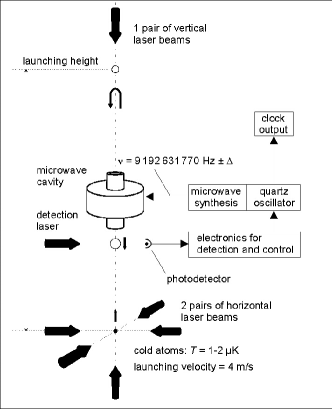
Figure 1: Schematic of an atomic fountain clock.

Caesium clocks are the most accurate primary standards for time and frequency bauch-99 . The hyperfine splitting frequency between the $F=3$ and $F=4$ levels of the ${}^{2}S_{1/2}$ ground state of the ¹³³Cs atom at 9.192 GHz has been used for the definition of the SI second since 1967. In a so-called caesium fountain (see Fig. 1), a dilute cloud of laser cooled caesium atoms at a temperature of about 1 $\mu$K is launched upwards to initiate a free parabolic flight with an apogee at about 1 m above the cooling zone. A microwave cavity is mounted near the lower endpoints of the parabola and is traversed by the atoms twice – once during ascent, once during descent – so that Ramsey’s method of interrogation with separated oscillatory fields ramsey-99 can be realized. The total interrogation time being on the order of 0.5 s, a resonance linewidth of 1 Hz is achieved, about a factor of 100 narrower than in traditional devices using a thermal atomic beam from an oven. Selection and detection of the hyperfine state is performed via optical pumping and laser induced resonance fluorescence. In a carefully controlled setup, a relative uncertainty slightly below$1\cdot 10^{-15}$ can be reached in the realization of the resonance frequency of the unperturbed Cs atom. The averaging time that is required to reach this level of uncertainty is on the order of $10^{4}$ s. One limiting effect that contributes significantly to the systematic uncertainty of the caesium fountain is the frequency shift due to cold collisions between the atoms. In this respect, a fountain frequency standard based on the ground state hyperfine frequency of the ⁸⁷Rb atom at about 6.835 GHz is more favorable, since its collisional shift is lower by more than a factor of 50 for the same atomic density. With the caesium frequency being fixed by definition in the SI system, the ⁸⁷Rb frequency is therefore presently the most precisely measured atomic transition frequency rb-99 .

II.2 Single-Ion Trap

An alternative to interrogating atoms in free flight, and a possibility to obtain practically unlimited interaction time, is to store them in a trap. Ions are well suited because they carry electric charge and can be trapped in radio frequency ion traps (Paul traps paul-99 ) that provide confinement around a field-free saddle point of an electric quadrupole potential. This ensures that the internal level structure is only minimally perturbed by the trap. Combined with laser cooling it is possible to reach the so-called Lamb–Dicke regime where the linear Doppler shift is eliminated. A single ion, trapped in an ultrahigh vacuum is conceptually a very simple system that allows good control of systematic frequency shifts deh-99 . The use of the much higher, optical reference frequency allows one to obtain a stability that is superior to microwave frequency standards, although only a single ion is used to obtain a correction signal for the reference oscillator.

A number of possible reference optical transitions with a natural linewidth of the order of 1 Hz and below are available in different ions, such as Yb⁺ yb-99 and Hg⁺ hg-99 . These ions possess a useful level system, where both a dipole-allowed transition and a forbidden reference transition of the optical clock can be driven with two different lasers from the ground state. The dipole transition is used for laser cooling and for the optical detection of the ion via its resonance fluorescence. If a second laser excites the ion to the metastable upper level of the reference transition, the fluorescence disappears and every single excitation can thus be detected with practically hundred percent efficiency as a dark period in the fluorescence signal.

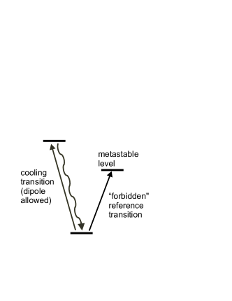
Figure 2: Double resonance scheme applied in single-ion-trap frequency standards.

Using these techniques and a femtosecond laser frequency comb generator (see Sect. 99.2.5) for the link to primary caesium clocks, the absolute frequencies of the transitions ${}^{2}S_{1/2}\rightarrow{{}^{2}D_{5/2}}$ in ¹⁹⁹Hg⁺ at 1065 THz and ${}^{2}S_{1/2}\rightarrow{{}^{2}D_{3/2}}$ in ¹⁷¹Yb⁺ at 688 THz have been measured with relative uncertainties of only $9\cdot 10^{-15}$. It is believed that single-ion optical frequency standards offer the potential to ultimately reach the $10^{-18}$ level of relative accuracy.

A similar double resonance technique can be employed if the reference transition is in the microwave domain and a number of accurate measurements of hyperfine structure intervals in trapped ions has been performed. In particular, the HFS interval in ¹⁷¹Yb⁺ has been measured several times ybhfs-99 and can be used to obtain constraints on temporal variations.

II.3 Laser-Cooled Neutral Atoms

Optical frequency standards have been developed with free laser-cooled neutral atoms, most notably of the alkaline-earth elements that possess narrow intercombination transitions. The atoms are collected in a magneto-optical trap, are then released and interogated by a sequence of laser pulses to realize a frequency-sensitive Ramsey-Bordé atom interferometer borde-99 . Of these systems, the one based on the ${}^{1}S_{0}\rightarrow{{}^{3}P_{1}}$ intercombination line of ⁴⁰Ca at 657 nm has reached the lowest relative uncertainty so far (about $2\cdot 10^{-14}$) hg-99 ; ca-99 . Limiting factors in the uncertainty of these standards are the residual linear Doppler effect and phase front curvature of the laser beams that excite the ballistically expanding atom cloud. It has therefore been proposed to confine the atoms in an optical lattice, i.e., in the array of interference maxima produced by several intersecting, red-detuned laser beams katori-99 . The detuning of the trapping laser could be chosen such that the light shift it produces in the ground and excited state of the reference transition are equal, and therefore it would produce no shift of the reference frequency. This approach is presently being investigated and may be applied to the very narrow (mHz natural linewidth) ${}^{1}S_{0}\rightarrow{{}^{3}P_{0}}$ transitions in neutral strontium, ytterbium, or mercury.

II.4 Two-Photon Transitions and Doppler-Free Spectroscopy

The linear Doppler shift of an absorption resonance can also be avoided if a two-photon excitation is induced by two counterpropagating laser beams. A prominent example that has been studied with high precision is the two-photon excitation of the $1S\rightarrow 2S$ transition in atomic hydrogen. The precise measurement of this frequency is of importance for the determination of the Rydberg constant and as a test of quantum electrodynamics (QED). Hydrogen atoms are cooled by collisions in a cryogenic nozzle and interact with a standing laser-wave of 243 nm wavelength inside a resonator. Since the atoms are not as cold as in laser cooled samples, a correction for the second order Doppler effect is performed. The laser excitation is interrupted periodically and the excited atoms are detected in a time resolved manner so that their velocity can be examined. An accuracy of about $2\cdot 10^{-14}$ has been obtained in absolute frequency measurements with a transportable caesium fountain h-99 .

II.5 Optical Frequency Measurements

In recent years, the progress in stability and accuracy of optical frequency standards has been impressive; and there is belief that in the future an optical clock may supersede the microwave clocks because the optical oscillators offer a much higher number of periods in a given time. In addition, some systematic effects, such as the Zeeman effect, have an absolute order of magnitude that does not scale with the transition frequency, and consequently is relatively less important at higher transition frequencies. A long-standing problem, however, was the precise conversion of an optical frequency to the microwave domain, where frequencies can be counted electronically in order to establish a time scale or can easily be compared in a phase coherent way.

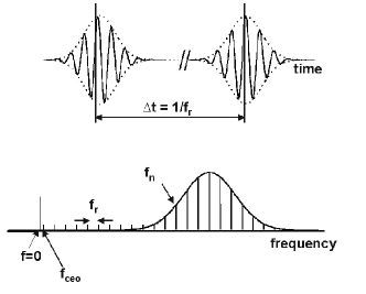
Figure 3: Frequency comb generated from femtosecond laser pulses.

This problem has recently been solved by the so-called femtosecond laser frequency comb generator chain-99 . Briefly, a mode-locked femtosecond laser produces, in the frequency domain, a comb of equally spaced optical frequencies $f_{n}$ that can be written as $f_{n}=nf_{r}+f_{\rm ceo}$ (with $f_{\rm ceo}<f_{r}$), where $f_{r}$ is the pulse repetition rate of the laser, the mode number $n$ is a large integer (of order $10^{5}$), and $f_{\rm ceo}$ (carrier-envelope-offset) is a shift of the whole comb that is produced by group velocity dispersion in the laser. The repetition rate $f_{r}$ can easily be measured with a fast photodiode. In order to determine $f_{\rm ceo}$, the comb is broadened in a nonlinear medium so that it covers at least one octave. Now the second harmonic of mode $n$ from the “red” wing of the spectrum, at frequency $2(nf_{r}+f_{\rm ceo})$, can be mixed with mode $2n$ from the “blue” wing, at frequency $2nf_{r}+f_{\rm ceo}$, and $f_{\rm ceo}$ is obtained as a difference frequency. In this way, the precise relation between the two microwave frequencies $f_{r}$ and $f_{\rm ceo}$ and the numerous optical frequencies $f_{n}$ is known. The setup can now be used for an absolute optical frequency measurement by referencing $f_{r}$ and $f_{\rm ceo}$ to a microwave standard and recording the beat note between the optical frequency $f_{\rm o}$ to be measured and the closest comb frequency $f_{n}$. Vice versa, the setup may work as an optical clockwork, for example, by adjusting $f_{\rm ceo}$ to zero and by stabilizing one comb line $f_{n}$ to $f_{\rm o}$ so that $f_{r}$ is now an exact subharmonic to order $n$ of $f_{o}$. The precision of these transfer schemes has been investigated and was found to be so high that it will not limit the performance of optical clocks for the foreseeable future.

II.6 Limitations on Frequency Variations

The frequency standards described above have been succesfully developed and their accuracy has been improved in the last decade. This progress, as a consequence, has led to certain constraints on the possible variations of the fundamental constants. Considering frequency variations, one has to have in mind that not only the numerical value but also the units may vary. For this reason, one needs to deal with dimensionless quantities which are unit-independent. During the last decade, a number of transition frequencies were measured in the corresponding SI unit, the hertz. These dimensional results are actually related to dimensionless quantities since a frequency measurement in SI is a measurement with respect to the caesium hyperfine interval

$$\bigl{\{}f\bigr{\}}=9\,192\,631\,770\;\mbox{}\cdot\frac{f}{f_{\rm HFS}({\rm Cs})}\;,$$ (1)

where $\bigl{\{}f\bigr{\}}$ stands for the numerical value of the frequency $f$. In Sect. IV, in order to simplify notation, this symbol for the numerical value is dropped.

Table 1: Limits on possible time variation of frequencies of different transitions in SI units. Here $\delta f/f$ is the fractional uncertainty of the most accurate measurement of the frequency $f$.

Atom,	$f$	$\delta f/f$	$\Delta f/\Delta t$	Refs.
transition	[GHz]	$[10^{-15}]$	[Hz/yr]
H, Opt	2 466 061	$14$	$-8\pm 16$	h-99
Ca, Opt	455 986	$13$	$-4\pm 5$	ca-99
Rb, HFS	6.835	$1$	$(0\pm 5)\cdot 10^{-6}$	rb-99
Yb+, Opt	688 359	$9$	$-1\pm 3$	ybnew-99
Yb+, HFS	12.642	$73$	$(4\pm 4)\cdot 10^{-4}$	ybhfs-99
Hg+, Opt	1 064 721	$9$	$0\pm 7$	hg-99

III Atomic spectra and the fundamental constants

III.1 The Spectrum of Hydrogen and Nonrelativistic Atoms

The hydrogen atom is the simplest atom and one can easily calculate the leading contribution to different kinds of transitions in its spectrum (cf., for example, Ref. here:Sapirstein-99 ), such as the gross, fine, and hyperfine structure. The scaling behavior of these contributions with the values of the Rydberg constant $R_{\infty}$, the fine structure constant $\alpha$, and the magnetic moments of proton and Bohr magneton is clear. The results for some typical hydrogenic transitions are

$$f(2p\to 1s) \simeq \frac{3}{4}\cdot cR_{\infty}\;,$$

$$f(2p_{3/2}-2p_{1/2}) \simeq \frac{1}{16}\cdot\alpha^{2}\cdot cR_{\infty}\;,$$

$$f_{\rm HFS}(1s) \simeq \frac{4}{3}\cdot\alpha^{2}\cdot\frac{\mu_{\rm p}}{\mu_{\rm B}}\cdot cR_{\infty}\;.$$ (2)

In the nonrelativistic approximation, the basic frequencies and the fine and hyperfine structure intervals of all atomic spectra have a similar dependence on the fundamental constants. The presence of a few electrons and a nuclear charge of $Z\neq 1$ makes theory more complicated and introduces certain multiplicative numbers but involves no new parameters. The importance of this scaling for a search for the variations was first pointed out in Ref. savedoff-99 and was applied to astrophysical data. Similar results may be presented for molecular transitions (electronic, vibrational, rotational and hyperfine) thompson-99 , however, up to now no measurement with molecules has been performed at a level of accuracy that is competitive with atomic transitions. They have been used only in a search for variations of constants in astrophysical observations (see e.g. varshalovich-99 ).

III.2 Hyperfine Structure and the Schmidt Model

The atomic hyperfine structure

$$f_{\rm NR}({\rm HFS})={\rm const}\cdot\alpha^{2}\cdot\frac{\mu}{\mu_{\rm B}}\cdot cR_{\infty}$$ (3)

involves nuclear magnetic moments $\mu$ which are different for different nuclei; thus, a comparison of the constraints on the variations of nuclear magnetic moments has a reduced value. To compare them, one may apply the Schmidt model (see, e.g., Ref. Karshenboim-99 ; sgk-99 ), which predicts all the magnetic moments of nuclei with an odd number of nucleons (odd value of atomic number $A$) in terms of the proton and neutron $g$-factors, $g_{\rm p}$ and $g_{\rm n}$, respectively, and the nuclear magneton only. Unfortunately, the uncertainty of the calculation within the Schmidt model is quite high (usually from 10% to 50%). The Schmidt model, being a kind of ab initio model, only allows for improvements which, unfortunately, involve some effective phenomenological parameters. This would not really improve the situation, but return us to the case where there are too many possibly varying independent parameters. A comparison of the Schmidt values to the actual data is presented for caesium, rubidium, and ytterbium in Table 2.

Table 2: Magnetic moments and relativistic corrections for atoms involved in microwave standards. The relativistic sensitivity $\kappa$ is defined in Sect. III.3. Here $\mu$ is an actual value of the nuclear magnetic moment, $\mu_{\rm N}$ is the nuclear magneton, and $\mu_{\rm S}$ stands for the Schmidt value of the nuclear magnetic moment; the nucleon $g$ factors are $g_{\rm p}/2\simeq 2.79$ and $g_{\rm n}/2\simeq-1.91$.

$Z$	Atom	$\mu/\mu_{\rm N}$	$\mu_{\rm S}/\mu_{\rm N}$	$\mu/\mu_{\rm S}$	$\kappa$
37	87Rb	2.75	$g_{\rm p}/2+1$	0.74	0.34
55	133Cs	2.58	$7/18\cdot(10-g_{\rm p})$	1.50	0.83
70	171Yb+	0.49	$-g_{\rm n}/6$	0.77	1.5

III.3 Atomic Spectra: Relativistic Corrections

A theory based on the leading nonrelativistic approximation may not be accurate enough. Any atomic frequency can be presented as

$$f=f_{\rm NR}\cdot F_{\rm rel}(\alpha)\;,$$ (4)

where the first (nonrelativistic) factor is determined by a scaling similar to the hydrogenic transitions (III.1). The second factor stands for relativistic corrections which vanish at $\alpha=0$; and thus, $F_{\rm rel}(0)=1$.

The importance of relativistic corrections for the hyperfine structure was first emphasized in Ref. prestage-99 . Relativistic many-body calculations for various transitions have been performed in Refs. flambaum04-99 ; dzuba1-99 ; dzuba01-99 ; dzuba03-99 . A typical accuracy is about 10%. Some results are summarized in Tables 2 and 3, where we list the relative sensitivity of the relativitic factors $F_{\rm rel}$ to changes in $\alpha$,

$$\kappa=\frac{\partial\ln F_{\rm rel}}{\partial\ln\alpha}\;.$$ (5)

Note that the relativistic corrections in heavy atoms are proportional to $(Z\alpha)^{2}$ because of the singularity of relativistic operators. Due to this, the corrections rapidly increase with the nuclear charge $Z$.

The signs and magnitudes of $\kappa$ are explained by a simple estimate of the relativistic correction. For example, an approximate expression for the relativistic correction factor for the hyperfine structure of an $s$-wave electron in an alkali-like atom is (see, e.g., Ref. prestage-99 )

$$F_{\rm rel}(\alpha)=\frac{1}{\sqrt{1-(Z\alpha)^{2}}}\cdot\frac{1}{1-(4/3)(Z\alpha)^{2}}\simeq 1+\frac{11}{6}(Z\alpha)^{2}\;.$$

A similar rough estimation for the energy levels may be performed for the gross structure:

$$E=-\frac{Z_{a}^{2}mc^{2}\alpha^{2}}{2n_{*}^{2}}\cdot\left(1+\frac{(Z\alpha)^{2}}{n_{*}}\frac{1}{j+1/2}\right)\;.$$ (6)

Here $j$ is the electron angular momentum, $n_{*}$ is the effective value of the principle quantum number (which determines the nonrelativistic energy of the electron), and $Z_{a}$ is the charge “seen” by the valence electron – it is 1 for neutral atoms, 2 for singly charged ions, etc. This equation tells us that $\kappa$, for the excitation of the electron from the orbital $j$ to the orbital $j^{\prime}$, has a different sign for $j>j^{\prime}$ and $j<j^{\prime}$. The difference of sign between the sensitivities of the ytterbium and mercury transitions in Table 3 reflects the fact that in Yb⁺ a $6s$-electron is excited to the empty $5d$-shell, while in Hg⁺ a hole is created in the filled $5d$-shell if the electron is excited to the $6s$-shell.

Table 3: Limits on possible time variation of the frequencies of different transitions and their sensitivity to variations in $\alpha$ due to relativistic corrections.

Atom, transition	$\partial f/f\partial t$	$\kappa$
H, $1s-2s$	$-3.2(63)\times 10^{-15}$ yr-1	0.	00
40Ca, ${{}^{1}}S_{0}-^{3}P_{1}$	$-8(11)\times 10^{-15}$ yr-1	0.	03
${}^{171}{\rm Yb}^{+}$, ${{}^{2}}S_{1/2}-{{}^{2}}D_{3/2}$	$-1.2(44)\times 10^{-15}$ yr-1	0.	9
${}^{199}{\rm Hg}^{+}$, ${}^{2}S_{1/2}-{{}^{2}}D_{5/2}$	$-0.2(70)\times 10^{-15}$ yr-1	$-3.$	2

IV Laboratory constraints on the variations of the fundamental constants

Logarithmic derivatives [see, e.g., Eq. (5)] appear since we are looking for a variation of the constants in relative units. In other words, we are interested in a determination of, e.g., $\Delta\alpha/\alpha\Delta t$ while the input data of interest are related to $\Delta f/f\Delta t$. Their relation takes the form

$$\frac{\partial\ln f}{\partial t}=\frac{\partial\ln f_{\rm NR}}{\partial t}+\kappa\cdot\frac{\partial\ln\alpha}{\partial t}\;.$$ (7)

If one compares transitions of the same type – gross structure, fine structure – the first term cancels.

IV.1 Constraints from Absolute Optical Measurements

Absolute frequency measurements offer the possibility to compare a number of optical transitions with frequencies $f_{\rm NR}$, which scale as $cR_{\infty}$, with the caesium hyperfine structure. One can rewrite Eq. (7) as

$$\frac{\partial\ln f_{\rm opt}}{\partial t}=\frac{\partial\ln cR_{\infty}}{\partial t}+\kappa\cdot\frac{\partial\ln\alpha}{\partial t}\;,$$ (8)

where dimensional quantities, such as frequency and the Rydberg constant, are stated in SI units [cf. Eq. (1)]. This equation may be used in different ways. For example, in Fig. 4 we plot experimental data for $\partial\ln f_{\rm opt}/\partial t$ as a function of the sensitivity $\kappa$ and derive a model-independent constraint on the variation of the fine structure constant

$$\frac{\partial\ln\alpha}{\partial t}=(-0.3\pm 2.0)\cdot 10^{-15}\,{\rm yr}^{-1}$$ (9)

and the numerical value of the Rydberg frequency $cR_{\infty}$ (see Table 4) in the SI unit of hertz. The latter is of great metrological importance, being related to a common drift of optical clocks with respect to a caesium clock, i.e., to the definition of the SI second. The SI definition of the metre is unpractical and so, in practice, the optical wavelengths of reference lines calibrated against the caesium standard are used to determine the SI metre quinn-99 .

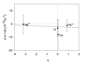
Figure 4: Frequency variations versus their sensitivity $\kappa$.

The constraints on the variations of $\alpha$ and $cR_{\infty}$ are correlated and the standard uncertainty ellipse, defined as

$$\sum_{i}\frac{1}{u_{i}^{2}}\left(\frac{\partial\ln f_{i}}{\partial t}-\frac{\partial\ln Ry}{\partial t}-\kappa_{i}\frac{\partial\ln\alpha}{\partial t}\right)^{2}=1+\chi^{2}_{\rm min}\,,$$

is presented in Fig. 5. Here we sum over all available data: $\partial\ln f_{i}/\partial t$ is the central value of the observed drift rate, $u_{i}$ its $1\sigma$ uncertainty, and $\chi^{2}_{\rm min}$ the minimized $\chi^{2}$ of the fit.

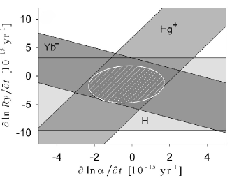
Figure 5: Constraints on the time variations of the fine structure constant $\alpha$ and the numerical value of the Rydberg constant. The preliminary data on Ca are not included.

The numerical value of the Rydberg constant, from the point of view of fundamental physics, can be expressed in terms of the caesium hyperfine interval in atomic units and its variation may be expressed in terms of the variations of $\alpha$ and $\mu_{\rm Cs}/\mu_{\rm B}$. A constraint for the latter is presented in Table 4.

IV.2 Constraints from Microwave Clocks

A model-independent comparison of different HFS transitions is not simple because their nonrelativistic contributions $f_{\rm NR}$ are not the same, but involve different magnetic moments. Applying Eq. (9) to experimental data, one can obtain constraints on the relative variations of the magnetic moments of Rb, Cs, and Yb (see Table 4).

Table 4: Model-independent laboratory constraints on the possible time variations of natural constants.

$X$	$\partial\ln X/\partial t$
$\alpha$	$(-0.3\pm 2.0)\cdot 10^{-15}\,{\rm yr}^{-1}$
$\{cR_{\infty}\}$	$(-2.1\pm 3.1)\cdot 10^{-15}\,{\rm yr}^{-1}$
$\mu_{\rm Cs}/\mu_{\rm B}$	$(3.0\pm 6.8)\cdot 10^{-15}\,{\rm yr}^{-1}$
$\mu_{\rm Rb}/\mu_{\rm Cs}$	$(-0.2\pm 1.2)\cdot 10^{-15}\,{\rm yr}^{-1}$
$\mu_{\rm Yb}/\mu_{\rm Cs}$	$(3\pm 3)\cdot 10^{-14}\,{\rm yr}^{-1}$

IV.3 Model-Dependent Constraints

In order to gain information on constants more fundamental than the nuclear magnetic moments, any further evaluation of the experimental data should involve the Schmidt model, which is far from perfect. Model-dependent constraints are summarized in Table 5.

Table 5: Model-dependent laboratory constraints on possible time variations of fundamental constants. The uncertainties here do not include uncertainties from the application of the Schmidt model.

$X$	$\partial\ln X/\partial t$
$m_{\rm e}/m_{\rm p}$	$(2.9\pm 6.2)\cdot 10^{-15}\,{\rm yr}^{-1}$
$\mu_{\rm p}/\mu_{\rm e}$	$(2.9\pm 5.8)\cdot 10^{-15}\,{\rm yr}^{-1}$
$g_{\rm p}$	$(-0.1\pm 0.5)\cdot 10^{-15}\,{\rm yr}^{-1}$
$g_{\rm n}$	$(3\pm 3)\cdot 10^{-14}\,{\rm yr}^{-1}$

The nucleon $g$ factors, in their turn, depend on a dimensionless fundamental constant $m_{\rm q}/\Lambda_{\rm QCD}$, where $m_{\rm q}$ is the quark mass and $\Lambda_{\rm QCD}$ is the quantum chromodynamic (QCD) scale. A study of this dependence may supply us with deep insight into the possible variations of the more fundamental properties of Nature (see Ref. flambaum04-99 for details). This approach is promising, but its accuracy needs to be better understood.

V Summary

The results collected in Tables 4 and 5 are competitive with data from other searches and have a more reliable interpretation. The results from astrophysical searches and the study of the samarium resonance from Oklo data claim higher sensitivity (see, e.g., Ref. book-99 ), however, they are more difficult to interpret. We have, for example, not assumed any hierarchy in variation rates or that some constants stay fixed while others vary, as it is done in the study of the position of the Oklo resonance. The evaluation presented here is transparent, and any particular calculation or measurement can be checked. In contrast, the astrophysical data show significant results only after an intensive statistical evaluation.

The laboratory searches involving atomic clocks have definitely shown progress and in a few years we expect an increase in the accuracy of these clocks, an increase in the number of different kinds of frequency standards (e.g., optical Sr, Sr⁺, In⁺ standards and a microwave Hg⁺ standard are being tried now), and indeed an increase in the time separation between accurate experiments, since it is now typically only 2–3 years. An optical clock based on a nuclear transition in Th-229 is also under consideration th229-99 . Such a clock would offer different sensitivity to systematic effects, as well as to variations of different fundamental constants.

Laboratory searches are not necessarily limited by experiments with metrological accuracy. An example of a high-sensitivity search with a relatively low accuracy is the study of the dysprosium atom for a determination of the splitting between the $4f^{10}5d6s$ and $4f^{9}5d^{2}6s$ states, which offers a great sensitivity value of $\kappa\simeq 5.7\cdot 10^{8}$ dzuba03-99 .

Variations of constants on the cosmological time scale can be expected but the magnitude, as well as other details, is unclear. Because of a broad range of options there is a need for the development of as many different searches as possible, and the laboratory search for variations is an attractive opportunity to open up a way that could lead to new physics.

Acknowledgments

We are very grateful to our colleagues and to participants of the ACFC-2003 meeting for useful and stimulating discussions.

References

- (1) W. E. Baylis and G. W. F. Drake, Chap. 1 in this Handbook.
- (2) P. J. Mohr and B. N. Taylor, Rev. Mod. Phys. (2004), to be published.
- (3) S. G. Karshenboim, Eprints physics/0306180 and physics/0311080, to be published.
- (4) Astrophysics, Clocks and Fundamental Constants, Lecture Notes in Physics, edited by S. G. Karshenboim and E. Peik (Springer, Berlin, 2004), Vol. 648.
- (5) N. F. Ramsey, Rev. Mod. Phys. 62, 541 (1990).
- (6) A. Bauch, H. R. Telle, Rep. Prog. Phys. 65, 789 (2002).
- (7) H. Marion, F. Pereira Dos Santos, M. Abgrall, S. Zhang, Y. Sortais, S. Bize, I. Maksimovic, D. Calonico, J. Gruenert, C. Mandache, P. Lemonde, G. Santarelli, Ph. Laurent, A. Clairon, and C. Salomon, Phys. Rev. Lett. 90, 150801 (2003).
- (8) W. Paul, Rev. Mod. Phys. 62, 531 (1990). See also: J. Javanainen, Chap. 73 in this Handbook.
- (9) H. Dehmelt, IEEE Trans. Instrum. Meas. 31, 83 (1982).
- (10) J. Stenger, C. Tamm, N. Haverkamp, S. Weyers, and H. R. Telle, Opt. Lett. 26, 1589 (2001).
- (11) T. Udem, S. A. Diddams, K. R. Vogel, C. W. Oates, E. A. Curtis, W. D. Lee, W. M. Itano, R. E. Drullinger, J. C. Bergquist, and L. Hollberg, Phys. Rev. Lett. 86, 4996 (2001); S. Bize, S. A. Diddams, U. Tanaka, C. E. Tanner, W. H. Oskay, R. E. Drullinger, T. E. Parker, T. P. Heavner, S. R. Jefferts, L. Hollberg, W. M. Itano, D. J. Wineland, and J. C. Bergquist, Phys. Rev. Lett. 90, 150802 (2003).
- (12) P. T. Fisk et al., IEEE Trans. UFFC 44, 344 (1997); P. T. Fisk, Rep. Prog. Phys. 60, 761 (1997); R. B. Warrington, P. T. H. Fisk, M. J. Wouters, and M. A. Lawn, in Proceedings of the 6th Symposium Frequency Standards and Metrology, edited by P. Gill (World Scientific, 2002), p. 297.
- (13) C. J. Bordé, Phys. Lett. A 140, 10 (1989).
- (14) G. Wilpers et al. , Phys. Rev. Lett. 89, 230801 (2002); F. Riehle et al. in Ref. book-99 , p. 229.
- (15) H. Katori, M. Takamoto, V. G. Pal’chikov, and V. D. Ovsiannikov, Phys. Rev. Lett. 91, 173005 (2003).
- (16) M. Niering, R. Holzwarth, J. Reichert, P. Pokasov, Th. Udem, M. Weitz, T. W. Hänsch, P. Lemonde, G. Santarelli, M. Abgrall, P. Laurent, C. Salomon, and A. Clairon, Phys. Rev. Lett. 84, 5496 (2000); M. Fischer et al., Phys. Rev. Lett. 92, 230802 (2004).
- (17) T. Udem, J. Reichert, R. Holzwarth, S. Diddams, D. Jones, J. Ye, S. Cundiff, T. W. Hänsch, and J. Hall, in The hydrogen atom: Precision physics of simple atomic systems, Lecture Notes in Physics, edited by S. G. Karshenboim et al. (Springer, Berlin, 2001), Vol. 570, p. 125.
- (18) E. Peik, B. Lipphardt, H. Schnatz, T. Schneider, Chr. Tamm, and S. G. Karshenboim, physics/04021132.
- (19) J. Sapirstein, Chap. 28 in this Handbook; P. Mohr, Chap. 29 in this Handbook.
- (20) M. P. Savedoff, Nature 178, 688 (1956).
- (21) R. I. Thompson, Astrophys. Lett. 16, 3 (1975).
- (22) D. A. Varshalovich, A. V. Ivanchik, A. V. Orlov, A. Y. Potekhin, and P. Petitjean, in Precision Physics of Simple Atomic Systems. Lecture Notes in Physics, edited by S. G. Karshenboim and V. B. Smirnov (Springer-Verlag, Berlin, 2003), Vol. 627, p. 199.
- (23) S. G. Karshenboim, Can. J. Phys. 78, 639 (2000).
- (24) V. V. Flambaum, physics/0309107; V. V. Flambaum, L.B. Leinweber, A.W. Thomas, and R.D. Young, Phys. Rev. D 69, 115006 (2004).
- (25) J. D. Prestage, R. L. Tjoelker, and L. Maleki, Phys. Rev. Lett. 74, 3511 (1995).
- (26) V. A. Dzuba, V. V. Flambaum, and J. K. Webb, Phys. Rev. Lett. 82, 888 (1999); Phys. Rev. A 59, 230 (1999).
- (27) V. A. Dzuba, V. V. Flambaum, Phys. Rev. A 61, 034502 (2001).
- (28) V. A. Dzuba, V. V. Flambaum, M.V. Marchenko, Phys. Rev. A 68, 022506 (2003).
- (29) T. J. Quinn, Metrologia 40, 103 (2003).
- (30) E. Peik and Chr. Tamm, Europhys. Lett. 61, 181 (2003).