A 15.2 TFlops Simulation of Geodynamo on the Earth Simulator

Abstract

For realistic geodynamo simulations, one must solve the magnetohydrodynamic equations to follow time development of thermal convection motion of electrically conducting fluid in a rotating spherical shell. We have developed a new geodynamo simulation code by combining the finite difference method with the recently proposed spherical overset grid called Yin-Yang grid. We achieved performance of 15.2 Tflops ($46\%$ of theoretical peak performance) on 4096 processors of the Earth Simulator.

I Introduction

The magnetic compass points to the north since the Earth is surrounded by a dipolar magnetic field. In the 19th century, Gauss showed that the origin of this geomagnetic field resides in the Earth’s interior. It is now broadly accepted that the geomagnetic field is generated by a self-excited electric current in the Earth’s core, which is a double-layered spherical region of radius $r=3500$km. The inner part of the core, called the inner core (radius $1200$km), is iron in solid state, and the outer part, called the outer core (radius $r$: $1200\hbox{km}\leq r\leq 3500\hbox{km}$), is also iron but in liquid state due to the high temperature of the planetary interior. The electrical current is generated by magnetohydrodynamic (MHD) dynamo action—the energy conversion process from flow energy into magnetic energy—of the liquid iron in the outer core. This geodynamo phenomenon is the target of our simulation reported in this paper.

In the last few decades, computer simulation has emerged as a central research method for geodynamo study kono_2002 . From the beginning of this new and exciting simulation area, we have been making important contributions by combining large scale simulation and advanced visualization technology: demonstration of the strong magnetic field generation by MHD dynamo kageyama_1995 , physical mechanism of the dipole field generation kageyama_1997 , and spontaneous and repeated reversals of the dipole moment (north-south polarity) ochi_1999 ; kageyama_1999 ; li_2002 .

Recently, we have proposed a new grid system for spherical geometry based on the overset (or Chimera) grid methodology. We have applied this new spherical grid to geodynamo simulation. In this paper, we report the development of this new geodynamo simulation code and its performance on the Earth Simulator shingu_2002 ; yokokawa_2002 ; habata_2003 , of Japan Agency for Marine-Earth Science and Technology (JAMSTEC), Japan.

II Yin-Yang grid

Since the Earth’s outer core is a spherical shell region between the inner core and the mantle, we need a numerically efficient spatial discretization method for a spherical shell geometry in order to achieve high performance on massively parallel computers.

In our previous geodynamo simulations, we used a finite difference method based on the latitude-longitude grid in spherical polar coordinates with the radius $r$ ($r_{i}\leq r\leq r_{o}$), colatitude $\theta$ ($0\leq\theta\leq\pi$), and the longitude $\phi$ ($-\pi<0\leq\phi\leq\pi$). Due to the existence of the coordinate singularity and grid convergence near the poles of the latitude-longitude grid, we had to take special care at the poles and this inevitably degraded the numerical efficiency and the performance of our previous dynamo code.

Since the finite difference method is suitable for massively parallel computers, especially massively parallel vector supercomputers like the Earth Simulator, we have decided to further exploit the possibilities of the finite difference method in spherical geometries, and to explore a new spherical grid system as the base of the spherical finite difference method.

There is no grid mesh that is orthogonal all over a spherical surface and, at the same time, free of coordinate singularity or grid convergence problems. So, we decompose the spherical surface into subregions. The decomposition, or dissection, enables us to cover each subregion by a grid system that is individually orthogonal and singularity-free.

The dissection of the computational domain generates internal borders between the subregions. In the overset grid approach chesshire_1990 , the subdomains are permitted to partially overlap one another on their borders. The overset grid is also called an overlaid grid, or composite overlapping grid, or Chimera grid steger_1983 . It is now one of the most important grid techniques in computational aerodynamics.

Recently, we have proposed a new overset grid for spherical geometry kageyama_2004 . The grid is named “Yin-Yang grid” after the symbol for yin and yang in the Chinese philosophy of complementarity. The Yin-Yang grid is composed of two identical and complemental component grids. Compared with other possible spherical overset grids, the Yin-Yang grid is simple in its geometry as well as metric tensors. A remarkable feature of this overset grid is that the two identical component grids are combined in a complemental way with a special symmetry. The Yin-Yang grid has already been applied to a mantle convection simulation in a spherical shell geometry with detailed benchmark tests yoshida_2004 . The Yin-Yang grid has also been applied to simulations of the global circulation of the atmosphere, ocean, and their coupled system takahashi_2004 ; xindong_2004 ; komine_2004 ; ohdaira_2004 ; hirai_2004 .

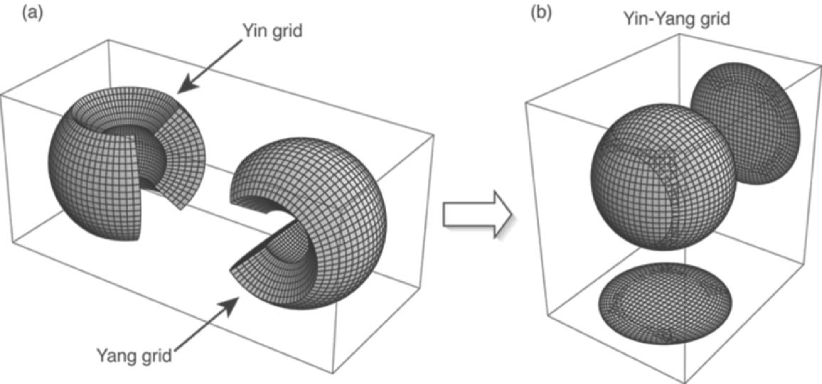
Figure 1: Basic Yin-Yang grid. The Yin grid and Yang grid are combined to cover a spherical surface with partial overlap.

There are several varieties of Yin-Yang grid kageyama_2004 . The most basic type, adopted in the geodynamo simulation reported in this paper, is shown in Fig. 1. It has two components—Yin and Yang—that are geometrically identical (exactly the same shape and size); see Fig. 1(a). We call the two component grids the “Yin grid” (or n-grid) and the “Yang grid” (or e-grid). They are combined to cover a spherical shell with partial overlap on their borders as shown in Fig. 1(b). Each component grid is, in fact, a part of the latitude-longitude grid on a spherical surface. (It is piled up in the radial direction). A component grid, say the Yin grid, is defined as a part of low-latitude region of the usual latitude-longitude grid: $90^{\circ}$ around the equator in latitude (between $45^{\circ}$N and $45^{\circ}$S), and $270^{\circ}$ in longitude. Another component grid, the Yang grid, is defined in the same way but in different spherical coordinates. The virtual north-south axis of the Yang grid is located on the equator of the Yin grid’s coordinates. The relation between Yin coordinates and Yang coordinates is written in Cartesian coordinates by

$$(x^{e},y^{e},z^{e})=(-x^{n},z^{n},y^{n}),\ \ \ \hbox{or}\ \ \ (x^{n},y^{n},z^{n})=(-x^{e},z^{e},y^{e}),$$ (1)

where $(x^{n},y^{n},z^{n})$ is the Yin grid’s Cartesian coordinates and $(x^{e},y^{e},z^{e})$ is Yang grid’s. Note that the forward and inverse transformations between Yin and Yang are given in the same form, which is a reflection of the complementary relation between the Yin and Yang grids.

It should be stressed that the Yin grid and Yang grid are identical in shape, geometry, grid, and metric tensors. This means that all subroutines designed for, say the Yin grid, can be used for the Yang grid with no modification. In addition to this geometrical symmetry, the Yin grid and Yang grid are in complementary coordinates relative to each other as indicated by eq. (1). This means that any interaction or communication from a grid point on Yin to a grid point on Yang is exactly the same as that from Yang to Yin. This fact makes the Yin-Yang-based computer code very concise and efficient.

Another advantage of the Yin-Yang grid resides in the fact that the component grid (Yin or Yang) is nothing but a (part of) latitude-longitude grid. This means that we can directly deal with the equations to be solved with the vector form in the usual spherical polar coordinates; components of a flow vector $\mathbf{v}$, for example, can be written as $\{v_{r},v_{\theta},v_{\phi}\}$ in the program. The analytical forms of metric tensors such as for Laplacian in spherical coordinates are well known. Since we can directly code the basic equations as they are formulated in spherical coordinates, we can make use of various resources of mathematical formulas, program libraries, and tools that have been developed in spherical polar coordinates.

Following the general overset methodology chesshire_1990 , interpolations are applied on the boundary of each component grid to set the boundary values, or internal boundary conditions. When one sees the component grid of the basic Yin-Yang grid shown in Fig. 1 in the Mercator projection, it is a rectangle; the four corners intrude most into the other component grid. Even if the grid mesh is taken to be infinitesimally small, the overlapping area has still non-zero ratio of about $6\%$ of the whole spherical surface. We obtain two solutions—one from the Yin side and other from the Yang side—in the overlapped area. This might be a slight ($6\%$) waste of computational time, but the “double solution” causes no problem in actual calculations. The difference between the two solutions is within the discretization error that is omnipresent on the sphere in any case. The difference between the solutions is so small that we do not need to “blend” the double solutions there in the post processing for the data visualization; we just choose one of the two solutions and the resulting visualization shows smooth pictures. There is no indication of the internal border between the Yin and Yang grids (e.g., Fig. 2 below).

If one still desires to minimize the overlapped area, it is possible by modifying the component grid’s shape from the rectangle. It is obvious that a Yin-Yang grid with a minimum overlap region can be constructed by a division, or dissection, using a closed curve on a sphere that cuts the sphere into two identical parts. There are infinite number of such dissections of a sphere. Two examples of them—“baseball type dissection” and “cube type dissection” can be found in kageyama_2004 .

III Basic equations and numerical methods

Since the physical model for the geodynamo simulation is the same as our previous one and described in our papers (e.g., kageyama_1995, ), here we describe it only briefly. We consider a spherical shell vessel bounded by two concentric spheres. The inner sphere of radius $r=r_{i}$ denotes the inner core and the outer sphere of $r=r_{o}$ denotes the core-mantle boundary. An electrically conducting fluid is confined in this shell region. Both the inner and outer spherical boundaries rotate with a constant angular velocity ${\bf\Omega}$. We use a rotating frame of reference with the same angular velocity. There is a central gravity force in the direction of the center of the spheres. The temperatures of both the inner and outer spheres are fixed; hot (inner) and cold (outer). When the temperature difference is sufficiently large, a convection motion starts when a random temperature perturbation is imposed at the beginning of the calculation. At the same time an infinitesimally small, random “seed” of the magnetic field is given.

The system is described by the following normalized MHD equations:

$$\frac{\partial\rho}{\partial t}=-\nabla\cdot\mathbf{f},$$ (2)

$$\frac{\partial\mathbf{f}}{\partial t}=-\nabla\cdot(\mathbf{v}\mathbf{f})-\nabla p+{\bf j}\times{\bf B}+\rho{\bf g}+2\rho{\bf v}\times{\bf\Omega}+\mu(\nabla^{2}{\bf v}+\frac{1}{3}\nabla(\nabla\cdot{\bf v})),$$ (3)

$$\frac{\partial p}{\partial t}=-\mathbf{v}\cdot\nabla p-\gamma p\nabla\cdot{\bf v}+(\gamma-1)K\nabla^{2}T+(\gamma-1)\eta{\bf j}^{2}+(\gamma-1)\Phi,$$ (4)

$$\frac{\partial{\bf A}}{\partial t}=-{\bf E},$$ (5)

with

$$p=\rho T,\hskip 30.00005pt{\bf B}=\nabla\times{\bf A},\hskip 30.00005pt{\bf j}=\nabla\times{\bf B},\hskip 30.00005pt{\bf E}=-{\bf v}\times{\bf B}+\eta{\bf j},$$

$${\bf g}=-g_{0}/r^{2}{\bf\hat{r}},\hskip 30.00005pt\Phi=2\mu\left(e_{ij}e_{ij}-\frac{1}{3}(\nabla\cdot{\bf v})^{2}\right),\hskip 30.00005pte_{ij}=\frac{1}{2}\left(\frac{\partial v_{i}}{\partial x_{j}}+\frac{\partial v_{j}}{\partial x_{i}}\right).$$ (6)

Here the mass density $\rho$, pressure $p$, mass flux density $\mathbf{f}$, magnetic field’s vector potential $\mathbf{A}$ are the basic variables in the simulation. Other quantities; magnetic field ${\bf B}$, electric current density ${\bf j}$, and electric field ${\bf E}$ are treated as subsidiary fields. The ratio of the specific heat $\gamma$, viscosity $\mu$, thermal conductivity $K$ and electrical resistivity $\eta$ are assumed to be constant. The vector ${\bf g}$ is the gravity acceleration and ${\bf\hat{r}}$ is the radial unit vector; $g_{0}$ is a constant. We normalize the quantities as follows: The radius of the outer sphere $r_{o}=1$; the temperature of the outer sphere $T(r_{o})$ = 1; and the mass density at the outer sphere $\rho(r_{o})=1$.

The spatial derivatives in the above equations are discretized by second-order central finite differences in spherical coordinates: ($r$, $\theta$, $\phi$). The fourth-order Runge-Kutta method is used for the temporal integration.

There are six free parameters—including three dissipation constants; viscosity $\mu$, thermal conductivity $K$, and electrical resistivity $\eta$—in this MHD system. We basically set the same parameter values adopted in our previous simulation that showed repeated dipole reversals li_2002 except for the three dissipation constants; we set each of them 10 times smaller than in the previous simulation. This means that the fluid’s Reynolds number and magnetic Reynolds number are both 10 times larger, the Rayleigh number—an index of the vigor of thermal convection—is 100 times larger, $3\times 10^{6}$, and the Ekman number is $2\times 10^{-5}$. Thus we can achieve more turbulent, and therefore more realistic simulations compared with our previous simulations.

IV Parallel Programming and Performance on the Earth Simulator

We have developed a new geodynamo simulation code (hereafter “yycore” code) for the Earth Simulator by converting our previous geodynamo code, which was based on the traditional latitude-longitude grid, into the Yin-Yang grid. We use the Fortran90 language and the MPI library. We make use of the module unit of Fortran90 to keep concise and neat program structure. All subroutines and functions are module subprograms. (There are no external subprograms.) In order to realize data hiding and encapsulation in the module level, we set the default attribute of module data and subprograms be private. The yycore code has about 6,200 lines of source (including comments). There are 12 modules and 1 main program. The total number of module-subprograms are 153. Among them, 48 subprograms are public (global scope).

We have found that the code conversion from our previous latitude-longitude-based code into the new Yin-Yang-based code is straightforward and rather easy. This is because most of the Yin-Yang grid code shares source lines with the latitude-longitude grid code: Our previous geodynamo code was basically a finite-difference MHD solver on spherical coordinates with a full span of colatitude $(0\leq\theta\leq\pi)$ and longitude $(-\pi<\phi\leq\pi)$; on the other hand, the Yin-Yang grid code (yycore) is also a finite-difference MHD solver on the spherical coordinates, but with just the smaller span of colatitude ($\pi/4\leq\theta\leq 3\pi/4$) and longitude ($-3\pi/4\leq\phi\leq 3\pi/4$). The major difference is the new boundary condition (interpolation) for the communication between Yin grid and Yang grid.

Our experience with the rapid and easy conversion from latitude-longitude code into Yin-Yang code should be encouraging for others who have already developed codes that are based on latitude-longitude grids in the spherical coordinates, and who are bothered by numerical problems and inefficiency caused by the pole singularity. We would like to suggest that they try the Yin-Yang grid.

Since the Yin grid and Yang grid are identical, dividing the whole computational domain into a Yin grid part and a Yang grid part is not only natural but also efficient for parallel processing. In addition to this Yin-and-Yang division, further domain decomposition within each grid is applied to achieve high performance on the Earth Simulator, a massively parallel computer.

The Earth Simulator, whose hardware specifications are summarized in Table I has three different levels of parallelization: vector processing in each arithmetic processor (AP); shared-memory parallelization by 8 APs in each processor node (PN); and distributed-memory parallelization by PNs.

In our yycore code, we apply vectorization in the radial dimension of the three-dimensional (3D) arrays for physical variables. The radial grid size is 255 or 511, which is just below the size (or doubled size) of the vector register of the Earth Simulator (256) to avoid bank conflicts in the memory shingu_2002 .

We use MPI both for the inter-node (distributed memory) parallel processing and for the intra-node (shared memory) parallel processing. This approach is called “flat-MPI” parallelization.

As we mentioned above, we first divide the whole computational domain into two identical parts—here we call them “panels”—that correspond to the Yin grid’s domain and the Yang grid’s domain in Fig. 1(a). In the yycore code, MPI_COMM_SPLIT is invoked to split the whole processes into two groups. (The total number of processes is even.) The world communicator is stored in a variable named gRunner%world%communicator, where gRunner is a nested derived type.

For further parallelization within a panel, there are several choices for the method of domain decomposition. Here we choose two-dimensional decomposition in the horizontal space, colatitude $\theta$ and longitude $\phi$, in each panel. For this purpose, we call MPI_CART_CREATE to make a two-dimensional process array with optimized rank order.

For the intra-panel communication, MPI_SEND and MPI_IRECV are called between nearest neighbor processes. Each process has four neighbors (north, east, south, and west). The rank numbers for the neighbors, obtained by invoking MPI_CART_SHIFT with the panel’s communicator gRunner%panel%communicator, are also stored in gRunner.

Communication between two groups (Yin and Yang) is required for the overset interpolation. This communication is implemented by MPI_SEND and MPI_IRECV under gRunner%world%communicator.

Peak performance of arithmetic processor (AP)	8 Gflops
Number of AP in a processor node (PN)	8
Total number of PN	640
Total number of AP	$8\hbox{ AP}\times 640\hbox{ PN}=5120$
Shared memory size of PN	16 GB
Total peak performance	$8\hbox{ Gflops}\times 5120\hbox{ AP}=40\hbox{Tflops}$
Total main memory	10TB
Inter-node data transfer rate	12.3 GB/s $\times$ 2

Table 1: Specifications of the Earth Simulator.

The best performance of yycore code with this flat MPI parallelization is $15.2$ Tflops. This number was obtained from the hardware counter for floating point operations on the Earth Simulator, which is automatically reported by setting the environment variable MPIPROGINF. This performance is achieved by $4096$ processors (512 nodes) with the total grid size of $511(\hbox{radial})\times 514(\hbox{latitudinal})\times 1538(\hbox{longitudinal})\times 2(\hbox{Yin and Yang})$. Since the theoretical peak performance of $4096$ processors is $4096\times 8\hbox{ Gflops}=32.8\hbox{Tflops}$, we have achieved $46\%$ of peak performance in this case. The average vector length is $251.6$, and the vector operation ratio is $99\%$. These data can be seen in the output of MPIPROGINF shown in List I. The high performance of the yycore code is a direct consequence of the simple and symmetric configuration design of the Yin-Yang grid: It makes it possible to minimize the communication time ($10\%$) between the processes in the horizontal directions, and enables optimum vector processing (with $99\%$ of operation ratio) in the radial direction in each process.

     MPI Program Information:
     ========================
     Note: It is measured from MPI_Init till MPI_Finalize.
           [U,R] specifies the Universe and the Process Rank in the Universe.

     Global Data of 4096 processes:          Min [U,R]             Max [U,R]         Average
     =============================

     Real   Time (sec)           :      452.157 [0,2623]      454.266 [0,680]       453.457
     User   Time (sec)           :      441.499 [0,1741]      447.001 [0,7]         443.220
     System Time (sec)           :        4.232 [0,455]         5.499 [0,9]           4.498
     Vector Time (sec)           :      321.969 [0,245]       380.540 [0,2138]      351.678
     Instruction Count           :  45628623153 [0,3152]  48004139033 [0,2]     46732455581
     Vector Instruction Count    :  13505506552 [0,855]   14116925576 [0,2178]  13758270302
     Vector Element Count        : 3395555533860 [0,1904] 3553256715628 [0,2178] 3461109543510
     FLOP Count                  : 1641123079258 [0,52]   1668645286059 [0,2178] 1642792822350
     MOPS                        :     7706.674 [0,7]        8102.270 [0,3938]     7883.403
     MFLOPS                      :     3671.412 [0,7]        3769.202 [0,1890]     3706.499
     Average Vector Length       :      250.582 [0,1120]      252.856 [0,4068]      251.564
     Vector Operation Ratio (%)  :       99.000 [0,7]          99.105 [0,3135]       99.056
     Memory size used (MB)       :     1042.944 [0,0]        1122.913 [0,9]        1106.882


     Overall Data:
     =============

     Real   Time (sec)           :      454.266
     User   Time (sec)           :  1815428.791
     System Time (sec)           :    18425.031
     Vector Time (sec)           :  1440471.743
     GOPS   (rel. to User Time)  :    32290.442
     GFLOPS (rel. to User Time)  :    15181.807         <--- 15.2 TFlops
     Memory size used (GB)       :     4427.528

List 1: An example of MPIPROGINF output.

To measure the performance dependency on the total number of processes, and the problem size (grid number), we executed several runs that are summarized in Table II.

processors	grid points	Tflops	efficiency
4096	$511\times 514\times 1538\times 2$	15.2	46%
3888	$511\times 514\times 1538\times 2$	13.8	44%
3888	$255\times 514\times 1538\times 2$	12.1	39%
2560	$511\times 514\times 1538\times 2$	10.3	50%
2560	$255\times 514\times 1538\times 2$	9.17	45%
1200	$255\times 514\times 1538\times 2$	5.40	56%

Table 2: Performance achieved by the yycore code—a finite difference geodynamo simulation program based on the Yin-Yang grid— on the Earth simulator.

Generally, flat MPI parallelization requires a larger problem size to achieve the same level of performance efficiency compared to the hybrid parallelization (e.g., MPI for inter-node and microtasking for intra-node parallelization) on the Earth Simulator nakajima_2002 . Since one Earth Simulator node has 8 APs (see TABLE I), the flat MPI method generates 8 times as many MPI processes as hybrid parallelization. However, in our yycore code with flat MPI, high performance could be achieved with relatively low numbers of mesh size: $15.2$ Tflops/512 PN with $511\times 514\times 1538\times 2=8\times 10^{8}$ grid points; $12.1$ Tflops/486 PN with $255\times 514\times 1538\times 2=4\times 10^{8}$ grid points. This can be compared with other flat MPI simulations on the Earth Simulator as reported in SC2002 and SC2003 (see Table III). Sakagami et al. sakagami_2002 achieved $14.9\hbox{ Tflops}/512\hbox{ PN}$ with $1.7\times 10^{10}$ grid points for a fluid simulation. (They used HPF to generate flat MPI processes.) Komatitsch et al. achieved $5\hbox{ Tflops}/243\hbox{ PN}$ with $5.5\times 10^{9}$ grid points komatitsch_2003 for seismic wave propagation. These results clealy indicate the high potential of the Yin-Yang grid as a base grid system on massively parallel computers.

Paper	Shingushingu_2002	Yokokawayokokawa_2002	Sakagamisakagami_2002	Komatitschkomatitsch_2003	Kageyama et al.
Flops/PN	26.6T/640	16.4T/512	14.9T/512	5T/243	15.2T/512
efficiency	65%	50%	45%	32%	46%
grid points (g.p.)	$7.1\times 10^{8}$	$8.6\times 10^{9}$	$1.7\times 10^{10}$	$5.5\times 10^{9}$	$8.1\times 10^{8}$
g.p./AP	$1.4\times 10^{5}$	$2.1\times 10^{6}$	$4.2\times 10^{6}$	$2.8\times 10^{6}$	$2.1\times 10^{5}$
Flops/g.p.	38K	19K	0.87K	0.91K	19K
Simulation kind	fluid	fluid	fluid	wave propagation	fluid
Field	atmosphere	turbulence	inertial fusion	seismic wave	geodynamo
Method	spectral	spectral	finite volume	spectral element	finite difference
Parallelization	MPI-microtask	MPI-microtask	HPF (flat MPI)	flat MPI	flat MPI

Table 3: Performances on the Earth Simulator reported at SC

V Simulation Results

For geodynamo study, it is necessary to follow the time development of the MHD system until the thermal convection flow and the dynamo-generated magnetic field are both sufficiently developed and saturated. (Initially, both the convection energy and the magnetic energy are negligibly small.) For the case of grid size of $255\times 514\times 1538\times 2=4\times 10^{8}$ with $3888$ processes, it took six hours of wall clock time until both the dynamo-generated magnetic field and convection flow energy reached to a saturated, and balanced, level. In normalized time units, this is about $0.3\%$ of the magnetic free decay time. This suggests that we need to integrate more time until we observe the dynamical features of the geodynamo such as the repeated dipole reversals ochi_1999 ; kageyama_1999 ; li_2002 .

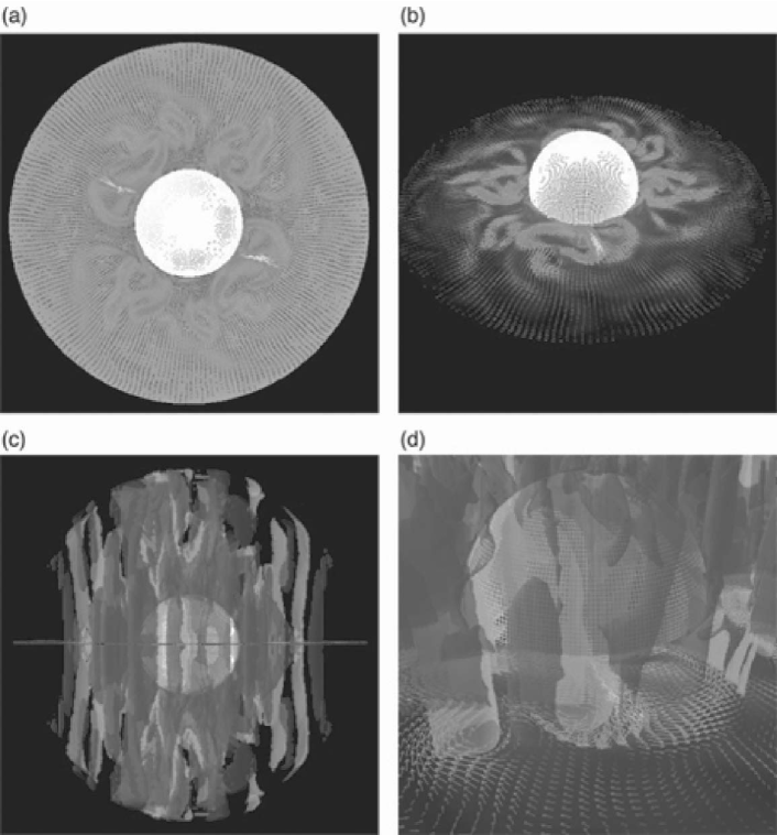
Figure 2: Thermal convection structure obtained by 3888 processor calculation on the Earth Simulator. The total grid size is $255(\hbox{radial})\times 514(\hbox{latitudinal})\times 1538(\hbox{longitudinal})\times 2(\hbox{Yin and Yang})$. In these visualizations, grid points are reduced by a factor of $1/100$. (a) Convection flow in the equatorial plane viewed from the north; (b) Same data as (a) but viewed from $45^{\circ}N$; (c) Columnar convection cells viewed in the equatorial plane. Two colors indicate cyclonic and anti-cyclonic convection columns; (d) Same data as (c), closer view.

As we described in Section III, the fundamental variables in our simulation are the magnetic vector potential $\mathbf{A}=\{A_{r},A_{\theta},A_{\phi}\}$, the mass flux density $\mathbf{f}=\{f_{r},f_{\theta},f_{\phi}\}$, pressure $p$, and the mass density $\rho$. It is convenient for data visualization/analysis purpose to store the Cartesian components of the magnetic field $\mathbf{B}=\{B_{x},B_{y},B_{z}\}$, velocity $\mathbf{v}=\{v_{x},v_{y},v_{z}\}$, vorticity $\mathbf{\omega}=\{\omega_{x},\omega_{y},\omega_{z}\}$, and temperature $T$. During one simulation run of 6 hours of wall clock time, we saved the 3-dimensional data 127 times, and about $500$ GB of data was generated in total.

It is known that thermal convection motion in a rapidly rotating spherical shell is organized as a set of columnar convection cells. The number of convection columns increases and the flow and the generated magnetic field becomes turbulent as shown in Fig. 2, which was obtained in the simulation of $3888$ processors with $255\times 514\times 1538\times 2$ grid points.

VI Summary

In this paper, we reported the development of a new geodynamo simulation code and presented its performance on the Earth Simulator. The base grid is the Yin-Yang grid, which is a spherical overset grid composed of two identical component grids. The achieved performance is 15.2 Tflops by 4096 processors with $511\times 514\times 1538\times 2$ grid points in a spherical shell.

- (1) G. Chesshire and W. D. Henshaw. Composite overlapping meshes for the solution of partial differential equations. J. Comput. Phys., 90:1–64, 1990.
- (2) Shinichi Habata, Mitsuo Yokokawa, and Shigemune Kitawaki. The Earth Simulator System. NEC Res. & Develop., 44(1):21–26, 2003.
- (3) Keisuke Hirai, Keiko Takahashi, Hidenori Aiki, Koji Goto, and Kunihiko Watanabe. Development of non-hydrostatic ocean circulation simulation code on the Earth Simulator. Proc. of The 2004 workshop on the solution of partial differential equations on the sphere, page 65, 2004.
- (4) A. Kageyama, T. Sato, K. Watanabe, R. Horiuchi, T. Hayashi, Y. Todo, T.H. Watanabe, and H. Takamaru. Computer simulation of a magnetohydrodynamic dynamo. II. Phys. Plasmas, 2:1421–1431, 1995.
- (5) Akira Kageyama, Marcia M. Ochi, and Tetsuya Sato. Flip-flop transitions of the magnetic intensity and polarity reversals in the magnetohydrodynamic dynamo. Phy. Rev. Lett., 82:5409–5412, 1999.
- (6) Akira Kageyama and Tetsuya Sato. Generation mechanism of a dipole field by a magnetohydrodynamic dynamo. Phys. Rev. E, 55:4617–4626, 1997.
- (7) Akira Kageyama and Tetsuya Sato. The “Yin-Yang Grid”: An overset grid in spherical geometry. Geochem. Geophys. Geosys., in press; preprint: arXive:physics/0403123, 2004.
- (8) Dimitri Komatitsch, Seiji Tsuboi, Chen Ji, and Jeroen Tromp. A 14.6 billion degrees of freedom, 5 teraflops, 2.5 terabyte earthquake simulation on the Earth Simulator. Proceedings of the ACM/IEEE Supercomputing SC’2003 conference, 2003, 2003.
- (9) Kenji Komine, Keiko Takahashi, and Kunihiko Watanabe. Development of a global non-hydrostatic simulation code using yin-yang grid system. Proc. of The 2004 workshop on the solution of partial differential equations on the sphere, pages 67–69, 2004.
- (10) Masaru Kono and Paul H. Roberts. Recent geodynamo simulations and observations of the geomagnetic field. Rev. Geophys., 40:1013, 2002.
- (11) Jinghong Li, Tetsuya Sato, and Akira Kageyama. Repeated and sudden reversals of the dipole field generated by a spherical dynamo action. Science, 295:1887–1890, 2002.
- (12) Kengo Nakajima. Three-level hybrid vs. flat MPI on the Earth Simulator: Parallel iterative solvers for unstructured grids on GeoFEM platform. RIST/TOKYO GeoFEM Report, 2002-007, 2002.
- (13) Marcia M. Ochi, Akira Kageyama, and Tetsuya Sato. Dipole and octapole field reversals in a rotating spherical shell: Magnetohydrodynamic dynamo simulation. Physics of Plasmas, 6:777–787, 1999.
- (14) Mitsuru Ohdaira, Keiko Takahashi, and Kunihiko Watanabe. Validation for the solution of shallow water equations in spherical geometry with overset grid system. Proc. of The 2004 workshop on the solution of partial differential equations on the sphere, page 71, 2004.
- (15) Hitoshi Sakagami, Hitoshi Murai, Yoshiki Seo, and Mitsuo Yokokawa. 14.9 TFLOPS three-dimensional fluid simulation for fusion science with HPF on the Earth Simulator. Proceedings of the ACM/IEEE Supercomputing SC’2002 conference, 2002.
- (16) Satoru Shingu, Hiroshi Takahara, Hiromitsu Fuchigami, Masayuki Yamada, Yoshinori Tsuda, Wataru Ohfuchi, Yuji Sasaki, Kazuo Kobayashi, Takashi Hagiwara, Shin ichi Habata, Mitsuo Yokokawa, Hiroyuki Itoh, and Kiyoshi Otsuka. A 26.58 Tflops global atmospheric simulation with the spectral transform method on the Earth Simulator. Proceedings of the ACM/IEEE Supercomputing SC’2002 conference, 2002.
- (17) Joseph L. Steger, F. Carroll Dougherty, and John A. Benek. A Chimera grid scheme. Advances in Grid Generation, edited by K.N. Ghia and U. Ghia:59–69, 1983.
- (18) Keiko Takahashi et al. Development of nonhydrostatic coupled ocean-atmosphere simulation code on the earth simulator. Proc.of 7th International Conference on High Performance Computing and Grid in Asia Pacific Region, Omiya, Japan, 2004.
- (19) Peng Xindong, Feng Xiao, Keiko Takahashi, and Takashi Yabe. Conservative CIP transport in meteorological model. JSME International Journal, to be published, 2004.
- (20) Mitsuo Yokokawa, Ken’ichi Itakura, Atsuya Uno, Takashi Ishihara, and Yukio Kaneda. 16.4-tflops direct numerical simulation of turbulence by a Fourier spectral method on the earth simulator. Proceedings of the ACM/IEEE Supercomputing SC’2002 conference, 2002.
- (21) Masaki Yoshida and Akira Kageyama. Application of the Yin-Yang grid to a thermal convection of a Boussinesq fluid with infinite Prandtl number in a three-dimensional spherical shell. Geophys. Res. Lett., 31:doi:10.1029/2004GL019970, 2004.