A Muon Collider Scheme Based on Frictional Cooling

Abstract

Muon Colliders would usher in a new era of scientific investigation in the field of high energy particle physics. The cooling of muon beams is proving to be the greatest obstacle in the realization of a Muon Collider. Monte Carlo simulations of a muon cooling scheme based on Frictional Cooling were performed. Critical issues, which require further study, relating to the technical feasibility of such a scheme are identified. Frictional Cooling, as outlined in this paper, provides sufficient six-dimensional emittance to make luminous collisions possible. It holds exciting potential in solving the problem of Muon Cooling.

1 Introduction

1.1 Motivation for a Muon Collider

The principal motivation for building a Muon Collider is to extend the high energy frontier of lepton colliders. With LEP, we likely have reached the maximum energy achievable with a circular electron collider, i.e., about $100$ GeV/beam. The limitation is the energy lost each turn through synchrotron radiation, which scales as $(E/m)^{4}$, where $E$ is the energy of the beam and $m$ is the mass of the particle. A linear electron-positron collider is currently under consideration which will operate at energies of $\leq 500$ GeV per beam. Reaching these energies requires very high electric fields as well as very long accelerators. Barring a breakthrough in acceleration techniques, it is difficult to see how much higher energies will be possible.

A Muon Collider could reach much higher energies in a circular accelerator since $m_{\mu}\approx 206~{}m_{e}$. Collisions between point-like particles would then be possible at energies similar to those achievable for proton accelerators, thus reopening the energy frontier with lepton colliders. The physics case for a high energy Muon Collider has been reviewed in many places. A recent compilation can be found in [1].

A significant additional benefit of a Muon Collider would be the intense and well understood flux of neutrinos resulting from muon decays allowing long baseline neutrino oscillation experiments to be performed with high statistics. The Collider complex could also be designed in such a way that neutrino scattering physics programs could be pursued. The physics case for a Neutrino Factory has been studied extensively and detailed accelerator studies are underway [2]. Low energy muons have a wide range of physics applications [3] which could also be pursued if the intense muon source required for the Muon Collider were constructed.

1.2 Difficulties

An obvious difficulty for the construction of a Muon Collider is the short muon lifetime ($2.2$ $\mu$s). Muons are not readily available and must be produced with a multi-MW proton source. Once the muons are produced, they occupy a very large phase space which must be reduced. The time available for this process is too short for existing techniques to be applicable (i.e.; stochastic cooling, synchrotron radiation damping rings). A new technique is required to reduce the muon emittance in a very short time. A related problem is that of backgrounds resulting from muon decays. Muon decays at all stages of the accelerator complex will produce radiation levels which will pose significant challenges for the accelerator elements. Any detector used to study the muon collisions will also see a large background flux from upstream muon decays. Of particular importance for a high energy, high current, muon beam is the radiation hazard resulting from the subsequent neutrino beam, which cannot be shielded [4].

1.3 Muon Cooling

Many of the difficulties listed above could be reduced with very effective muon cooling. Cooler beams would allow fewer muons for a given luminosity, and thereby reduce the experimental backgrounds, reduce the radiation from muon decays, reduce the radiation from neutrino interactions, and allow for smaller apertures in the accelerator elements. Fewer required muons would also be welcome for the targetry and proton driver, which provide severe technical and financial constraints. We therefore identify the efficient cooling of the muon beam phase space as the signature challenge for a future Muon Collider.

2 Cooling Schemes

2.1 Overview of a Muon Collider Complex

Before briefly reviewing the proposed muon cooling schemes, we provide an overview of a possible Muon Collider complex along with beam parameters. Figure 1 shows schematically the different elements required for a Muon Collider.

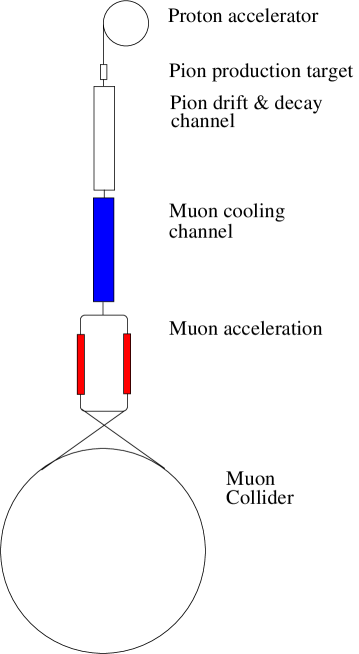
Figure 1: Schematic of a Muon Collider complex.

The first stage is a proton driver, which is a high intensity proton accelerator producing several MW of protons in the energy range $2-30$ GeV (different schemes have different optimal energies). The protons then impact a target in a region with a very strong magnetic field, and the resulting charged particles, primarily pions, are captured in a decay channel. The pion drift and decay channel is optimized to yield a maximum number of muons in the required energy range. The muons then enter a cooling channel where the phase space of the beam is compressed and they are then brought to the desired energy in a series of accelerators.

A parameter set for a 3 TeV center-of-mass (CoM) energy Muon Collider is given in [5], and is summarized in Table 1.

CoM energy (TeV)	3
proton energy (GeV)	16
protons/bunch	$2.5\cdot 10^{13}$
bunches/fill	4
Rep. rate (Hz)	15
$\mu$/bunch	$2\cdot 10^{12}$
collider circ. (m)	6000
$\epsilon_{6,N}(\pi{\rm m})^{3}$	$1.7\cdot 10^{-10}$
Luminosity (cm-2s-1)	$7\cdot 10^{34}$

Table 1: A set of parameters for a 3 TeV CoM energy Muon Collider [5].

The required normalized six-dimensional emittance for this parameter set is $\epsilon_{6,N}=1.7\cdot 10^{-10}$ in units of $({\pi{\rm m}})^{3}$. At the end of the pion drift and decay channel, the RMS dimensions of the muon cloud in spatial coordinates x, y, z are approximately 0.05, 0.05, 10 m, and in momentum coordinates $P_{x},P_{y},P_{z}$ are $50,50,100$ MeV/c, yielding $\epsilon_{6,D}=1.7\cdot 10^{-4}({\pi{\rm m}})^{3}$. The required emittance reduction is therefore of order $10^{6}$, and this reduction must be accomplished with a reasonable efficiency.

To reach the luminosities given in Table 1, $0.08~{}\mu$ per $16$ GeV proton must be in the cooled phase space for each muon charge. If we fix the power of the proton driver at $4$ MW, then we aim for $0.01$ muons of each sign per $2$ GeV proton, which is our optimal proton beam energy (see section 4.1.2).

The cooling scheme which has received considerable consideration is Ionization Cooling. We describe this briefly in the next section. The cooling scheme we have chosen to investigate, Frictional Cooling, is then broadly outlined. The remainder of this paper describes in more detail a conceptual design for the early stages of a Muon Collider based on Frictional Cooling. It should be understood as an attempt to find a solution to the cooling problem satisfying physical limitations such as muon lifetime, scattering effects and energy loss mechanisms. Technical feasibility has not been investigated.

2.2 Ionization Cooling

Ionization Cooling operates at kinetic energies of the order of 100 MeV. For a Muon Collider, emittance reduction would be achieved in alternating steps. First, transverse emittance cooling is achieved by lowering the muon beam energy in high density absorbers (such as liquid hydrogen) and then reaccelerating the beam to keep the average energy constant. Both transverse and longitudinal momenta are reduced in the absorbers, but only the longitudinal momentum is restored by the RF. In this way, transverse cooling can be achieved up to the limit given by multiple scattering. Second, longitudinal emittance cooling is achieved by adding dispersion into the muon beam and passing the momentum gradiented beam through wedge shaped absorbers such that the higher momentum muons pass through more absorber than the lower momentum muons. This process adds to the transverse emittance. The steps can then be repeated until the limits from multiple scattering are reached. The trade off between the transverse and longitudinal cooling portions is called emittance exchange and the resultant beam is cooled in six dimensions.

Although Ionization Cooling shows promise and has been investigated in detail [6], the simulation studies have yet to show the required emittance reduction to make a Muon Collider feasible. Various schemes based on Ionization Cooling have achieved six-dimensional emittance reductions of the order of 100-200 [7].

3 Frictional Cooling

3.1 Basic Idea

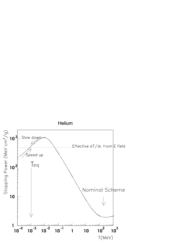
Figure 2: The stopping power, $\frac{1}{\rho}dT/ds$, in Helium as a function of kinetic energy, $T$, for $\mu^{+}$ (solid line). The effective stopping power resulting from an external electric field is sketched as a dotted line. An equilibrium kinetic energy, $T_{eq}$, near $1$ keV would result. The nominal scheme discussed for a Neutrino Factory, based on Ionization Cooling, would cool muons near $T=200$ MeV.

The basic idea of Frictional Cooling [8] is to bring the muons into a kinetic energy range, $T$, where energy loss per unit path length, $ds$, increases with kinetic energy. A constant accelerating force is then applied to the muons resulting in an equilibrium kinetic energy. A sample $\frac{1}{\rho}dT/ds$ curve is shown in Fig. 2, where it is seen that this condition can be met for kinetic energies below a few keV, or kinetic energies beyond about $200$ MeV. At the high energy end, the change in $dT/ds$ with energy is only logarithmic, whereas it is approximately proportional to speed at low energies. We focus on the region below the ionization peak. In this region, ionization is suppressed because the relative speed between the muon and orbital electrons is too low to allow sufficient transfer of kinetic energy for ionization.

3.2 Some Difficulties & Solutions

We study the low energy regime where $dT/ds$ is proportional to the speed $v$ and $v\leq\alpha c$, where $\alpha$ is the fine structure constant. In this energy regime, we imagine applying an electric field which compensates $dT/ds$, yielding an equilibrium kinetic energy. Several issues are immediately apparent:

• $\frac{1}{\rho}dT/ds$ is very large in this region of kinetic energy, so we need to work with a low average density material in order to have a reasonable electric field strength, $|\vec{E}|$. Efficiency considerations lead to the use of a gas rather than a system with alternating high and low densities, such as foils. We could tolerate larger electric fields in a system of foils. However, the foils will give larger energy loss fluctuations, resulting in problems with $\mu^{-}$ capture and muonium (bound state of $\mu^{+}$ and electron) formation. In addition, a large fraction of the muons would be stopped in the foils and subsequently lost. We therefore pursue the use of a gas volume with a strong electric field to extract the muons.

• The lifetime of the $\mu^{\pm}$ can be written as

  $$v\tau\approx 0.1\sqrt{T(eV)}\;\;{\rm m}\;\;\;\;\;T\ll m_{\mu}c^{2}\;.$$

  The muons should therefore only travel tens of centimeters at the low kinetic energies to have a significant survival probability. They must then be reaccelerated quickly to avoid loss due to decay.

• A strong solenoidal field, $\vec{B}$, will be needed to guide the muons until the beams are cooled. We cannot have $\vec{E}$, in the cooling cell, parallel to $\vec{B}$ or the muons will never get below the peak of the $dT/ds$ curve. The muons will have typical kinetic energies well above the $dT/ds$ peak when they enter the gas volume. The electric field strength required to balance $dT/ds$ at the low energies would produce a strong acceleration of the muons at these high initial kinetic energies, such that the muons never slow down. We therefore consider an electric field transverse to the magnetic field. In the cooling cell, the force on a muon is given by

  $$\vec{F}=q(\vec{E}+\vec{v}\times\vec{B})-\frac{dT}{ds}\hat{v},$$

  where $\hat{v}$ is a unit vector in the direction $\vec{v}$. At the higher energies, the muons follow the magnetic field lines with slow drift and pick up minimal energy from the electric field. Once the muons have slowed down, however, the electric force is no longer small compared to the magnetic force and the muons will drift out of the volume at a definite Lorentz angle. In this way, the cooling cell can be long in the initial direction of the beam and short in the transverse direction in which the beam is extracted.

• Large electric fields generally will result in breakdown in gases. Having $\vec{E}\perp\vec{B}$ is expected to avoid this problem by limiting the maximum kinetic energy an ionized electron can acquire and thus prevent charge multiplication.

• Muonium (Mu) formation ($\mu^{+}+{\rm Atom}\rightarrow{\rm Mu}+{\rm Atom}^{+}$) is significant at $\mu^{+}$ energies near the ionization peak. In fact, the muonium formation cross section dominates over the electron stripping cross section in all gases except Helium [9]. This leads us therefore to choose Helium as a stopping medium (at least for $\mu^{+}$).

• For $\mu^{-}$, a possibly fatal problem is the loss of muons resulting from muon capture, $\mu^{-}+{\rm Atom}\rightarrow\mu{\rm Atom}+e^{-}$. The cross section for this process has been calculated up to kinetic energies of about $80$ eV [10, 11], at which point the cross section, for H₂ and Helium, is of order $10^{-17}$ cm², and falling rapidly. Cross sections of order $10^{-21}$ cm² are necessary for the cooling described here to have significant efficiency for $\mu^{-}$. Large capture cross sections extend to higher $T$ for higher atomic number $Z$. To maximize the yield of $\mu^{-}$, we therefore need to use a low $Z$ material and keep the kinetic energy as high as possible. Helium or Hydrogen appear to be the best choices for the $\mu^{-}$ slowing medium.

• At the low energies used in Frictional Cooling, the question of extracting muons from any gas cell becomes a significant issue. The use of very thin windows as a possible solution will be discussed in section 7.1.

• Intense ionization from the slowing muons will produce a large number of free charges which will screen the applied $\vec{E}$ field. The speed at which this happens and the extent of the field reduction have not been studied and will require further thought. It is briefly discussed in section 7.4.

3.3 Outline of a Scheme based on Frictional Cooling

We have investigated the scheme illustrated in Fig. 3.

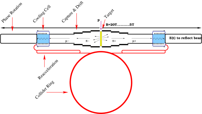
Figure 3: Overview of a Muon Collider based on Frictional Cooling. The different sections are not to scale.

Muons of both signs are produced by scattering an intense proton beam on a target located in a region with a very strong solenoidal magnetic field ($20$ T, as in the Neutrino Factory study). A drift region with a more moderate magnetic field, of the order of $5$ T, allows the bulk of the pions to decay to muons. The muons are then input into the cooling channel, which consists of a cooling cell roughly $\sim 11~{}$m long. The cooling cell contains Helium gas (possibly H₂ for $\mu^{-}$), and an electric field perpendicular to the magnetic field. The electric field direction is reversed periodically, as a function of the position along the axis of the gas cell, to cancel the beam drift. The muons stopped in the cell drift out at a characteristic angle dependent on ${\vec{B}}$ and ${\vec{E}}$. They are then extracted through thin windows and reaccelerated.

At the end of the drift region, there is a correlation between the longitudinal momentum of the muons and their arrival time. This allows for a phase rotation, where time varying electric fields are used to increase the number of muons at lower momenta. In contrast to schemes based on Ionization Cooling, the phase rotation section follows the cooling cell, such that those muons already in the low energy regime, which can achieve equilibrium in the medium, are not lost. In the following, we describe each of these elements and their simulations in more detail.

4 Simulation of the Collider Front End

The role of the target system for a Muon Collider is analogous to that of a Neutrino Factory. One needs to generate a maximal number of pions with an intense proton beam and then capture and guide them into a channel where they can decay to muons. The muons from the pion decays can then be cooled, reaccelerated and stored in a ring for subsequent injection into a collider. However, the evaluation criteria for optimizing the pion yield is different for the Neutrino Factory from that of a Muon Collider based on Frictional Cooling. By virtue of the low energy required for Frictional Cooling, the target system is optimized for the yield of low energy pions. The starting point was taken from the Feasibility Study II for the Neutrino Factory [2]. We then modified the design to fit our needs.

The following target yield studies were performed using the MARS Monte Carlo code [12]. MARS performs fast, inclusive simulations of three-dimensional hadronic and electromagnetic cascades, and performs muon and low energy neutron transport in material, in the energy range of a fraction of an eV up to 30 TeV. The subsequent transport of produced particles in the target area and decay channel was simulated using the GEANT 3.21 package [13]. The cooling and reacceleration simulation was performed with custom written code.

4.1 Targetry

The initial target geometry studied consisted of the Study II [2] target, in which the proton beam impinged a target under a small angle. A strong solenoidal field is used to capture pions in a wide phase space. The extraction of the pion beam takes place in the longitudinal direction (the direction of the incident proton beam) in the Neutrino Factory scheme.

This is not ideal for Frictional Cooling because the highest momentum muons, which result from decays of the highest momentum pions, would not be cooled. Frictional Cooling requires the optimization of the pion yield at low energies. Figure 4 shows the signed kinetic energy of the produced $\pi^{\pm}$ from the target.

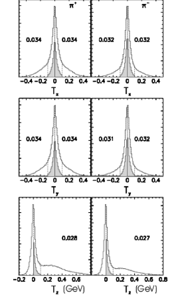
Figure 4: Signed kinetic energy (in units of GeV) of $\pi^{+}$ (left) and $\pi^{-}$ (right) produced at the target, for a 2 GeV proton beam on a $0.75~{}{\rm cm}\times 30~{}{\rm cm}$ Copper target. $T_{x,y,z}$ is defined as $\frac{P_{x,y,z}}{|P_{x,y,z}|}T_{x,y,z}$. The shaded histograms correspond to those pions with a kinetic energy less than 100 MeV. The vertical scale is arbitrary. The numbers on the plots indicate the number of pions per 1 GeV proton on target within the shaded regions.

The z-direction is the longitudinal or proton beam direction. The low energy pion yield transverse to the target is larger than that in the longitudinal direction. Moreover, there are relatively equal yields for $\pi^{+}$ and $\pi^{-}$. This allows the possibility to develop a symmetric $\mu^{+}$ and $\mu^{-}$ machine and hence cool both signs at the same time. We have therefore chosen to extract the pions produced transverse to the target. The magnetic field is therefore perpendicular to the direction of the proton beam.

4.1.1 Layout of Target Area

The pion capture mechanism consists of a solenoidal magnetic field channel starting with B=20 T near the target and falling adiabatically to 5 T at 18 m. Particle capture/extraction takes place transverse to the target or direction defined by the proton beam.

The magnetic field is symmetric with a gap for the non-interacting proton beam, and forward produced particles, to pass through. Figure 5 shows the dimensions of the solenoid coils and magnetic field profile.

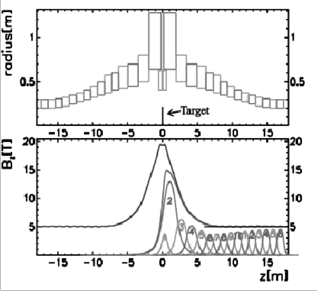
Figure 5: The upper plot shows schematically the arrangement, in cross section, of the solenoids used to create the tapered solenoidal field. The lower plot shows the contributions from individual solenoids and their cumulative field along the z axis. The target is represented by the solid line at z=0.

Note that the z-direction is redefined in this figure to the direction of extraction which is transverse to the target. The proton beam trajectory in this strong field has not been simulated in detail.

4.1.2 Optimization of Yields

An optimization of the composition and geometry of the target was performed to find the maximal pion yield, which would produce coolable muons. Coolable muons were defined as those with a kinetic energy less than 120 MeV. The target material, geometry and the energy of the proton driver, were varied to find the optimum yield. The results of this study are summarized in Fig. 6.

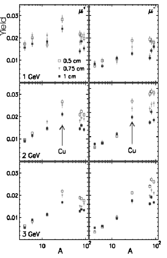
Figure 6: Yields of $\mu^{+}$ (left) and $\mu^{-}$ (right), in units of number of $\mu$ per 1 GeV p, as a function of the atomic mass of the target material for different target thicknesses as denoted by the symbols. The rows correspond to different proton driver beam energies; 1 GeV, 2 GeV and 3 GeV as denoted in the figures.

The choice of a Copper target resulted in the optimal yield. A Tungsten target produced similar performance and may be more desirable in terms of stability and target lifetime.

Figure 7 shows the effect of the proton driver beam energy on the yield for various target species and thicknesses.

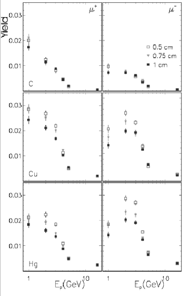
Figure 7: Yields of $\mu^{+}$ (left) and $\mu^{-}$ (right), in units of number of $\mu$ per 1 GeV p, as a function of the proton driver beam energy for different target thicknesses as denoted by the symbols. The rows correspond to different target materials; Carbon, Copper and Mercury as denoted in the figures.

A proton beam energy of 2 GeV results in the highest yield and roughly equal yield for both signs of pions. This is important in the development of a $\mu^{+}\mu^{-}$ collider.

4.2 Drift Region

The solenoidal field is tapered down from 20 T at the target to 5 T in order to reduce the amount of stored energy of such a section and to reduce cost. We have used a similar design to that given in [2]. The length over which the pion beams are allowed to drift and decay was then optimized (for the muon yield). Figure 8 shows the results of this study.

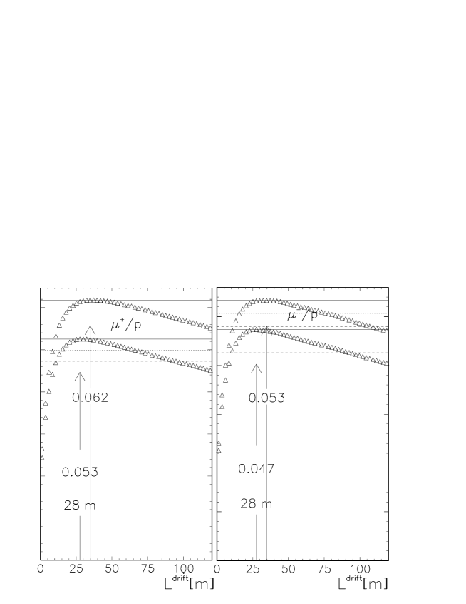
Figure 8: Yield as a function of decay channel length $L^{drift}$ for $\mu^{+}$ (left) and $\mu^{-}$ (right), in units of number of $\mu$ per 1 GeV p. The lower symbols indicate the number of $\mu$ per 1 GeV p with $T_{z}<120~{}$MeV.

The optimum drift length is taken to be the distance which gives the maximum $\mu^{+}/p$ yield for $T_{\mu^{+}}<120$ MeV and is found to be 28 m.

4.3 Summary of Target and Drift regions

In summary, the optimization of the front end of a muon Frictional Cooling scheme resulted in the following scenario:

• a 2 GeV proton driver

• a Copper target 30 cm in length and 0.5 cm thick

• a drift length of 28 m

The yield at the end of the drift of such a front end is $0.062~{}\mu^{+}$ per 2 GeV proton and $0.054~{}\mu^{-}$ per 2 GeV proton.

4.4 Phase Rotation Section

At the end of the cooling cell, there is a correlation between the longitudinal momentum of the muons which survive and the arrival time. This allows for a phase rotation to take place, where time varying electric fields are used to increase the number of muons at lower momenta. A simple ansatz was used for the phase rotation section and consisted of a flat 5 MV/m field for some time $t_{1}$, after which the field went linearly to zero at a time $t_{2}$. These parameters were optimized ($t_{1}=100$ ns and $t_{2}=439$ ns) to obtain the maximum number of muons/proton coming from the front end. The effect of the phase rotation on the kinetic energy distribution of the muons is shown in Fig. 9.

Figure 9: The kinetic energy, $T$, distributions for a $\mu^{+}$ beam before and after the phase rotation section. Both before and after distributions correspond to muons which are eventually cooled.

5 Cooling Cell

The simulated cooling cell is a cylinder filled with either Helium (for $\mu^{+}$ or $\mu^{-}$) or Hydrogen (for $\mu^{-}$) gas. The axis of the cylinder defines the z-direction (or longitudinal direction) and corresponds to the direction of the muon beam. The entrance windows at either end must pass $T\leq 50$ MeV muons with high efficiency. The extracted muons come out transversely and have low energy. The windows for the transverse extraction must have high efficiency for $T\leq 1$ keV muons.

The gas cell consists of one continuous volume, 11 m in length. The cell is located immediately after the drift region to capture those muons which are already slow enough to be stopped in 11 m of gas. The bulk of the muons at higher energies pass unaffected through the gas cell into the phase rotation section. The phase rotation reflects the beam using time changing electric fields and is optimized to produce a maximum number of muons at low kinetic energies such that they can be stopped in the gas cell.

The density of Helium used in the simulation for $\mu^{+}$ was $1.25\cdot 10^{-4}$ g/cm³, which corresponds to roughly 0.7 atm at STP. For $\mu^{-}$, 0.3 atm of He or H₂ was used, which correspond to densities of $5.35\cdot 10^{-5}$ and $2.5\cdot 10^{-5}$ g/cm³ respectively.

The window thicknesses for the extraction of low energy muons varied from 0-20 nm of Carbon. These windows are conceived as grids upon which a Carbon film is deposited. The grid would have a large open area ($>80\%$), and this loss in efficiency has not been simulated.

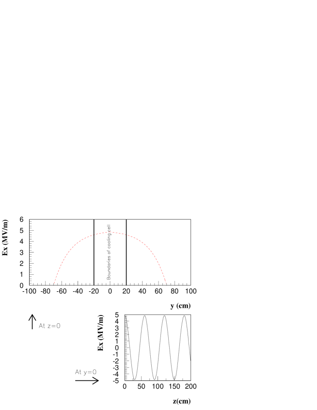
Figure 10: Variation of E_x inside the cooling cell region. The upper plot indicates the variation of E_x as a function of y at z=0 and the lower plot shows the variation of E_x as a function of z at y=0.

The entire cooling and phase rotation sections were contained inside a uniform 5 T solenoidal field and the crossed electric field strength was taken to be 5 MV/m inside the gas cell section. The electric field oscillated as a cosine function every 30 cm inside the gas cell and was exponentially damped to zero at a radius 70 cm. The E_x field profile is defined as follows,

$$E_{x}=E_{0}\cdot cos(z[{\rm cm}]\pi/30.)\cdot(1-exp(-(|y[{\rm cm}]|-70)/20)),$$

and can be seen in Fig. 10. The technical feasibility of such a field configuration has not yet been investigated.

5.1 Tracking

The physics processes are described in more detail in the next section - we focus here on the technical aspects of the tracking. Muon decay and muon capture were not simulated but were taken into account by calculating the probability that the muons survived these processes.

The tracking of muons proceeded as follows:

• The position of the muon was used to determine the local value of the electric and magnetic fields, as well as the local material and density.

• Given the muon momentum and the medium in which it was located, the mean free path to the next nuclear scatter was calculated. The mean free path was then used to generate a track step, $D$.

• $D$ was then compared to the maximum step size, $d$, (typically 10 $\mu$m), set to preserve accuracy in tracking. If $D>d$ then $D$ was broken up into several steps of size $\leq d$.

• The Runge-Kutta-Merson approach was then used to update the position and momentum of the muon according to the Lorentz force equation for each step using the CERN routine [14] DDEQMR. The force law included the continuous energy loss from scattering on electrons via:

  $$\vec{F}=\frac{d\vec{P}}{dt}=q\vec{E}+q\vec{v}\times\vec{B}-\frac{dT}{ds}\hat{v},$$

  where $T$ is the muon kinetic energy and $s$ is the path length. The total time was updated at each step, and the time interval in the step was used to update the decay survival probability. For negative muons, the capture survival probability was also updated based on the step length and kinetic energy.

• Once the full distance $D$ was reached, a scattering angle was generated according to the relevant differential cross section. The momentum components of the muon were then updated appropriately.

This procedure was followed until either the muon left the cooling cell volume or one of the survival probabilities fell below $0.001$. The tracking code was tested extensively and was found to give very accurate results. Examples of muon trajectories are given in section 5.2.

5.1.1 Simulation of Physics Processes

Frictional Cooling cools muon beams to the limit of nuclear scattering. A detailed simulation was therefore performed where all large angle nuclear scatters were simulated. The differential distributions and mean free paths for $\mu$-nucleus scattering were calculated in two different ways depending on the energy regime. A quantum mechanical (Born Approximation) calculation was used for the scattering cross section at high kinetic energies ($T_{\mu}>2$ keV) and a classical calculation was used at lower kinetic energies. The screened Coulomb potential used in the Born and classical calculations had the form

$$V=\frac{4e^{2}}{r}~{}exp(\frac{-r}{a}),$$

where $a$ is the screening length. For the classical calculation the procedure of Everhart et al. [15] was followed. The differential cross section was calculated by scanning in impact parameter and evaluating the scattering angle at each impact parameter. From the differential cross section, a mean free path for scattering angles greater than a cutoff (0.05 rad) was found, and scatters were then generated according to the differential cross section. This method reproduces the energy loss from nuclear scatters tabulated by NIST [16] for protons. The simulation results for $\mu^{+}$ and $\mu^{-}$ are shown in Fig. 11.

Figure 11: Energy loss from nuclear scattering or nuclear stopping power for $\mu^{+}$ and $\mu^{-}$ produced using the stand alone Monte Carlo.

For $\mu^{+}$, the electronic energy loss is taken from the NIST tables. The suppression for $\mu^{-}$ (Barkas effect [17]) was parameterized from the results in [18]. The electronic energy loss was treated as a continuous process. The electronic energy losses for $\mu^{+}$ and $\mu^{-}$ are shown in Fig. 12.

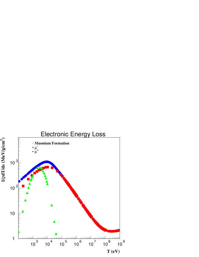
Figure 12: The electronic energy loss for $\mu^{+}$ and $\mu^{-}$. For comparison, the simulated energy loss due to muonium formation (see text) is also shown.

This difference is significant below the ionization peak, which is expected to be due in part to muonium formation.

To simulate the effect of muonium formation in the tracking, an effective charge was used, as given by $\sigma_{I}/(\sigma_{F}+\sigma_{I})$, where $\sigma_{I}$ is the cross section for muonium ionization and $\sigma_{F}$ is the cross section for muonium formation (see Fig. 13).

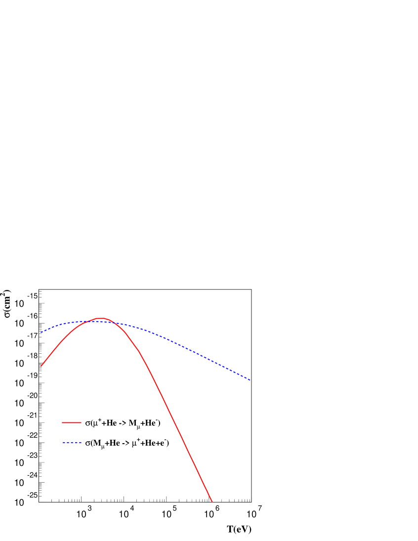
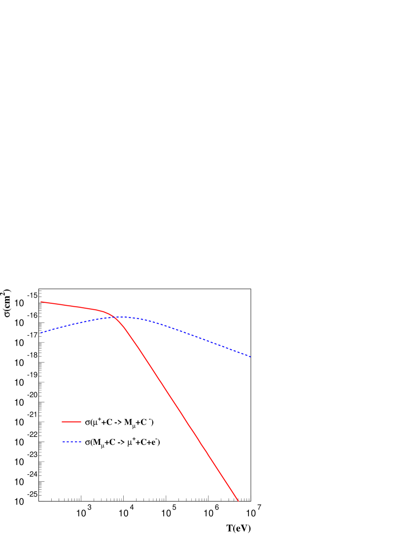
Figure 13: The muonium formation, $\sigma(\mu^{+}+{\rm A}\rightarrow M_{\mu}+{\rm A}^{-})$, and muonium ionization, $\sigma(M_{\mu}+{\rm A}\rightarrow\mu^{+}+{\rm A}+e^{-})$, cross sections for Helium (left) and Carbon (right) [9].

Negative muon capture was parameterized from calculations of Cohen [10, 11] and included in our simulation. The calculations only extend up to 80 eV. Beyond this, a simple exponential fall off with kinetic energy was assumed. The parameterization is plotted in Fig. 14.

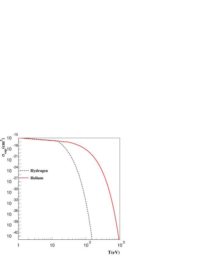
Figure 14: Parameterization of $\mu^{-}$ capture cross section, $\sigma_{\rm cap}$, in Hydrogen and Helium used in the simulation as a function of the kinetic energy of the $\mu^{-}$, $T$.

5.2 Trajectories

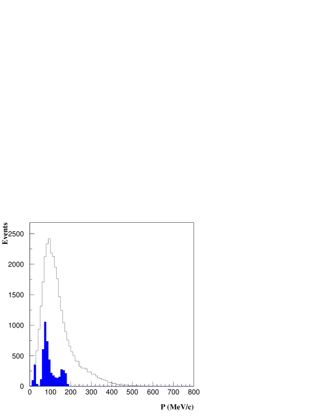
Figure 15: The momentum, $\vec{P}$, distribution of muons entering the cooling section (histogram). The distribution of those which result in cooled muons is shaded.

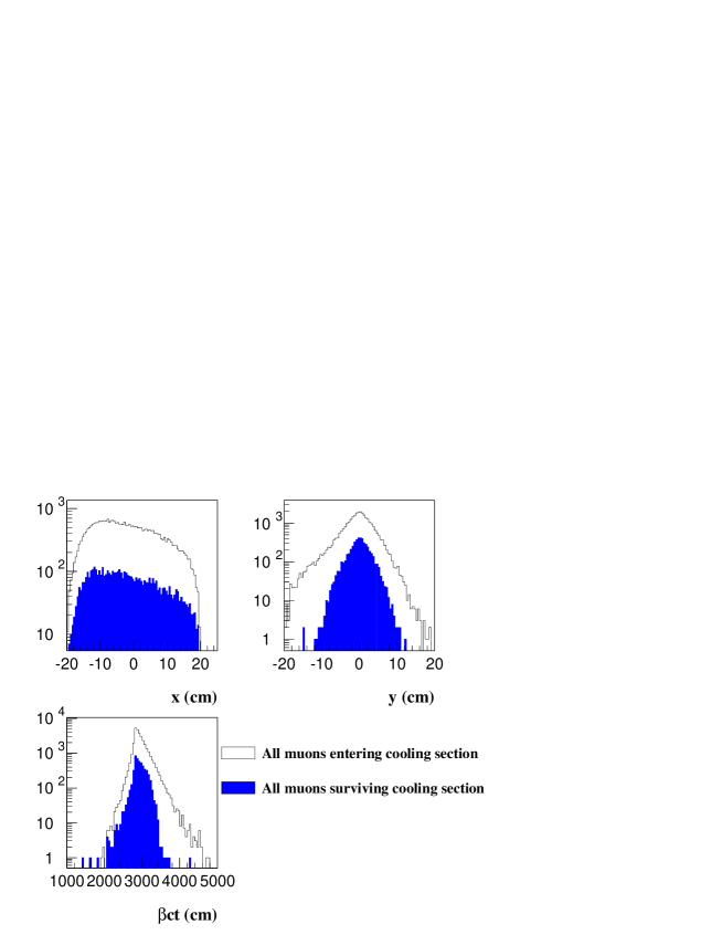
Figure 16: The transverse and longitudinal spatial distributions of muons entering the cooling section (histogram). The distributions of those which result in cooled muons is shaded. The top plots indicate the transverse, x and y, spatial distributions and the bottom plot shows the longitudinal spatial distribution expressed as $\beta ct$, where $\beta c$ is the muon velocity and $t$ is absolute time.

The momentum and space distributions of muons at the end of the decay channel are displayed in Fig. 15 and Fig. 16. The full histograms show the input distributions, while the shaded histograms show the distributions of muons which survive. From these distributions, one can see that this cooling channel does not cool muons with a momentum greater than 200 MeV/c. In the absence of electric and magnetic fields the range, in meters, for a $\mu^{+}$ in He gas with density $\rho=1\cdot 10^{-4}$ gm/cm³ was found to be

$$R~{}{\rm[m]}=1.2\cdot 10^{-4}(|\vec{P}|~{}{\rm[MeV/c]})^{3.35},$$

with the momentum given in units of (MeV/c). The cooling cell has a length of 11 m. Due to the transverse momentum of the muon, the total path length in the cell is on average 20 m. Therefore, muons with $\vec{P}\leq 35$ MeV/c will be stopped in the gas cell. This can either happen on the first pass (first peak in Fig. 15), or after the phase rotation/reflection (second and third peaks in Fig. 15). For the maximum momentum, muons require about $300$ ns to reach the equilibrium energy, $T_{eq}$. The time required to drift transversely out of the cell depends on where the muon reached $T_{eq}$. Taking as nominal values $T_{eq}=500$ eV and a drift distance of 20 cm (cell radius) yields an additional time of $200$ ns. Additional flight times appear for the muons which are reflected by the phase rotation section and in the initial reacceleration (described below). The time required for cooling the muons and extracting them is therefore of order $1$ $\mu$s.

We now describe example muon trajectories in different sections of the cooling cell. In Fig. 17, the path of a muon with initial momenta: $P_{x}=1~{}{\rm MeV/c},P_{y}=0~{}{\rm MeV/c}$ and $P_{z}=100~{}{\rm MeV/c}$ is shown in the yz and xy views.

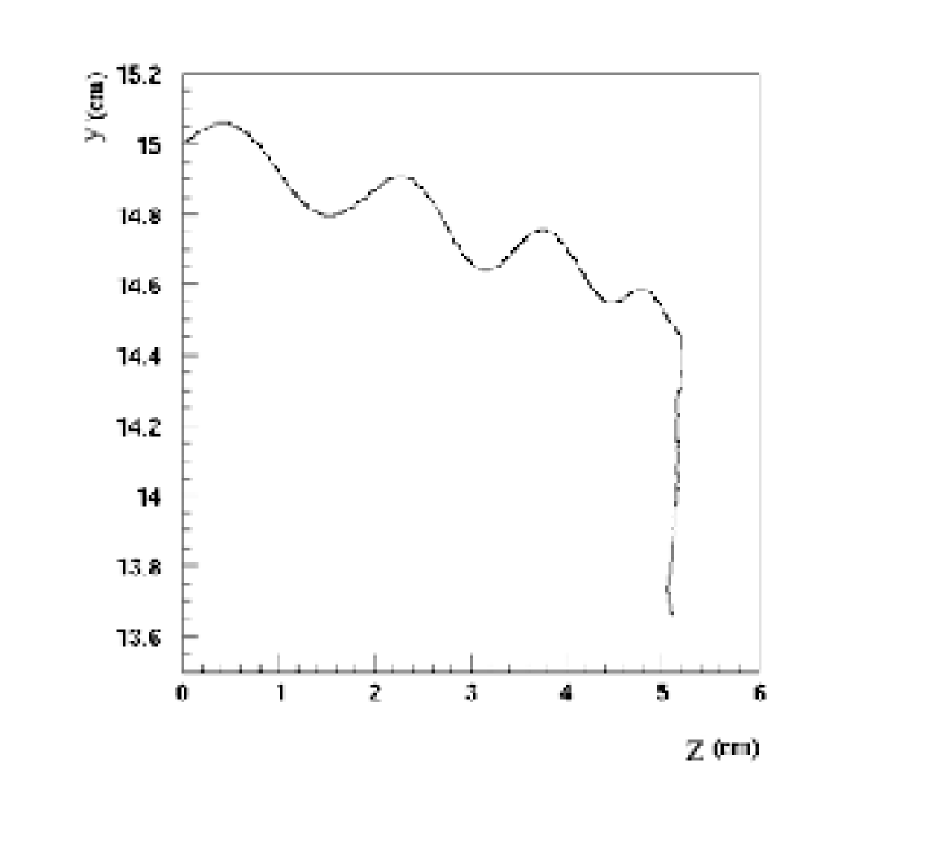
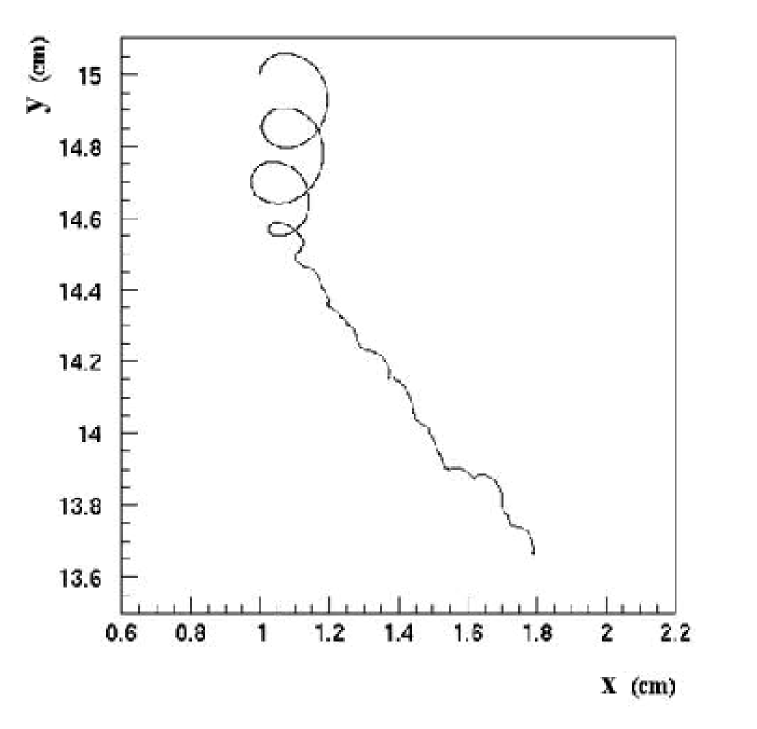
Figure 17: The yz (left) and xy (right) views of the final stages of the trajectory of a single muon in the cooling cell with initial momenta: $P_{x}=1~{}{\rm MeV},P_{y}=0~{}{\rm MeV}$ and $P_{z}=100~{}{\rm MeV}$.

In the yz view, the slow drift of the muon in the y direction resulting from the $\vec{E}\perp\vec{B}$ field is evident. Also, the radius of the trajectory is decreasing due to the energy loss in the gas. Once the muon has reached the equilibrium energy, it is extracted from the cell at a fixed Lorentz angle, which is clearly seen in the x-y plane view. The effect of the large angle nuclear scatters is visible. The effect on the kinetic energy of the muon is shown in Fig. 18, where the kinetic energy is plotted as a function of time.

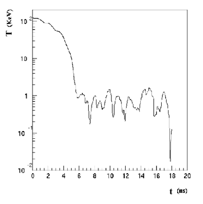
Figure 18: The kinetic energy, $T$, as a function of time, $t$, of the final stages of the trajectory of a muon in the cooling cell with initial momenta: $P_{x}=1~{}{\rm MeV/c},P_{y}=0~{}{\rm MeV/c}$ and $P_{z}=100~{}{\rm MeV/c}$.

The large oscillations in kinetic energy depend very strongly on the scattering angle. In some cases, the muon bounces off a nucleus in a direction opposite to the accelerating force. In this case, a muon can come almost to rest before it is reaccelerated. This is a particularly dangerous situation for $\mu^{-}$, since the capture probability increases rapidly at the smaller kinetic energies as shown in Fig. 14.

The muons can drift either in the positive-x or negative-x direction depending on the sign of the electric field in the region where it reached equilibrium energy. Once the muon reaches the edge of the cooling cell, it is extracted through a thin window and enters a completely evacuated region.

6 Acceleration and Bunching

6.1 Initial Reacceleration

Upon leaving the cooling cell, the extracted muons undergo cycloid motion with net direction of motion along the positive or negative-y direction. The parameters of the cycloid change adiabatically with the changing electric field as a function of y. For $|y|>30$ cm, an electric field component in the z-direction is also present,as shown in Fig. 19, so that muons are then accelerated along the z-axis.

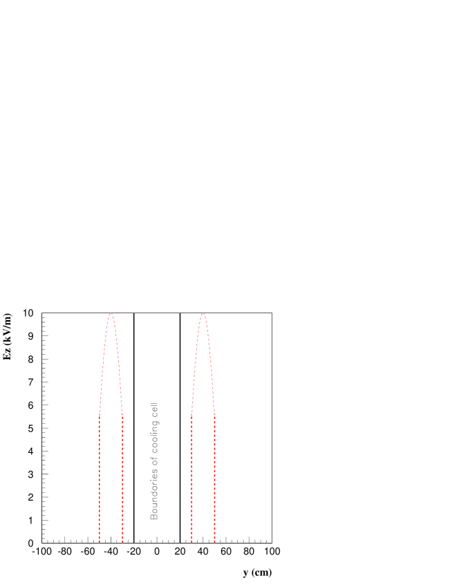
Figure 19: Variation of E_z as a function of y inside cooling cell region.

This electric field is relatively weak in order to avoid inducing too large a momentum spread in the beam at the end of the $11$ m section. The value of the z-coordinate at which muons are extracted from the gas cell is plotted in Fig. 20.

Figure 20: The distribution of the z position for the surviving muons extracted from the 11 m long cooling cell.

The distribution is rather flat, so that muons will have a relatively flat kinetic energy spectrum at the end of the $11$ m cell between $0$ and $0.11$ MeV.

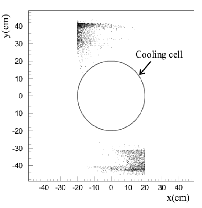
Figure 21: The x,y distribution of muons at z=11 m after the initial reacceleration.

The final beam position after this reacceleration is shown in Fig. 21. The muon beam has an arithmetic mean energy of $\sim 427$ keV and a root mean square of $\sim 306$ keV. The time spread of the beam coming out of this initial reacceleration is shown in Fig. 22 and has a root mean square of 1 $\mu$s.

Figure 22: The arrival time, $t$, distribution of muons at z=11 m after the initial reacceleration. $t=0$ is defined as the time when the proton beam hits the target.

The beam coming out of the initial reacceleration region must continue to be rapidly accelerated and, most importantly, the time spread reduced. Fig. 23 shows the results of a preliminary reacceleration. The effect on the time distribution is significant as the RMS of the time distribution goes from 1 $\mu$s to 3 ns whilst the momentum RMS spread increases from 1.2 MeV/c to 5 MeV/c at a final mean momentum of 147 MeV/c. The survival rate for this reacceleration is 30%.

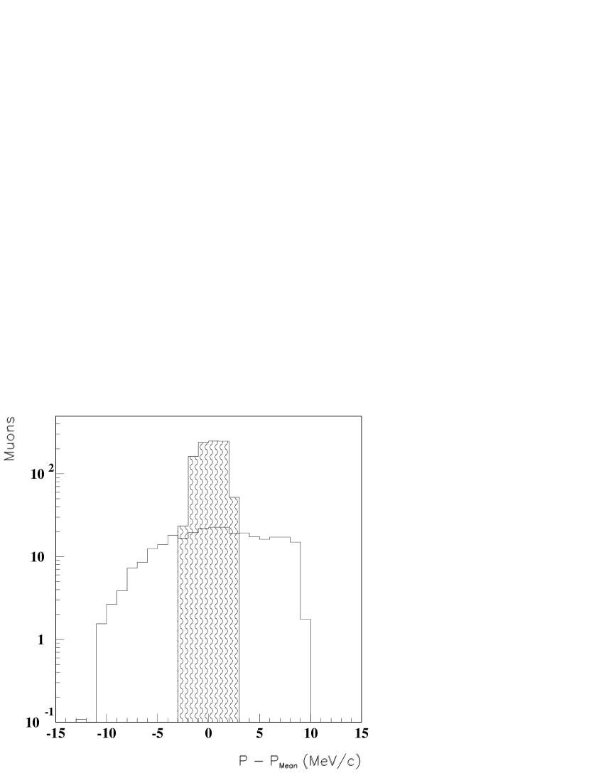
Figure 23: The momentum spread (left) and time spread (right) of the muon beam before (hatched histogram) and after (histogram) reacceleration.

6.2 Phase Space Reduction

The six-dimensional normalized emittance is calculated as follows:

$$\epsilon_{6D,N}=\frac{\sigma_{x}\sigma_{y}\sigma_{z}\sigma_{px}\sigma_{py}\sigma_{pz}}{(\pi~{}m_{\mu}c)^{3}},$$

where the $\sigma$’s are RMS values of the transverse and longitudinal components of the muon beam. The emittance is evaluated at a given z position of the beam and thus the $\sigma_{z}$ is calculated using $\sigma_{\beta ct}$ at a given z. In calculating the emittance no correlations are taken into account between the distributions. The total phase space reduction is calculated by taking the ratio ($\epsilon^{\prime}_{6D,N}/\epsilon^{0}_{6D,N}$) of the final, $\epsilon^{\prime}_{6D,N}$, and initial, $\epsilon^{0}_{6D,N}$, emittances of the muon beam. The initial emittance is calculated using the initial distributions of those muons which are successfully cooled. Another method would be to take the emittance calculated using all the muons at the end of the drift. However, there is an acceptance limitation for this channel - the channel cannot accept the entire beam produced by the front end of this scheme. This is evident since the initial emittance, calculated from the beam components given in Table 2, is smaller than the emittance of the entire muon beam at the end of the drift.

	$\mu^{+}$
x0 (cm)	9.48
y0 (cm)	2.68
$\beta_{0}$ c t0 (cm)	176.93
px0 (MeV/c)	20.24
py0 (MeV/c)	20.39
pz0 (MeV/c)	37.91
x (cm)	4.48/5.30
y (cm)	4.76/3.85
$\beta$ c t (cm)	1600.71/1612.02
px (MeV/c)	0.16/0.16
py (MeV/c)	0.15/0.16
pz (MeV/c)	1.18/1.22 7
yield ($\mu$/2 GeV p)	0.0021

Table 2: Initial and final RMS values for the six-dimensional ingredients of the emittance, and yields for $\mu^{+}$. The final numbers for $\mu^{+}$ include the extraction through a 20 nm thick Carbon window. x, y and $\beta$ c t are the spatial components, and px, py and pz are the momentum components of the muon beam. Those quantities with a suffix $0$ refer to the initial values of the muon beam and those without a suffix refer to the final values. Note that there are two values for each of the final components referring to the two beamlets which come out of this scheme.

This indicates that any pre-cooling channel which cools the beam by one order of magnitude could then be followed by such a frictional cooling channel and hence increase the yield of the entire scheme.

The results for the simulated scheme outlined in this report are listed in Tables 2 and 3.

Window thickness		1st Beamlet	2nd Beamlet
20 nm $\mu^{+}$	Initial	Final	Final
$\epsilon_{T,N}$ ($\pi$ m)2	9.51e-6	4.56e-10	4.71e-10
$\epsilon_{L,N}$($\pi$ m)	0.20	0.057	0.059
$\epsilon_{6D,N}$($\pi$ m)3	1.92e-6	2.61e-11	2.79e-11

Table 3: Normalized emittances for the initial and final muon beams for $\mu^{+}$.

The yield for this scheme is $0.0021~{}\mu^{+}$ per 2 GeV proton. This yield does not change greatly for window thicknesses up to 20 nm. As a consequence of the alternating transverse electric field there are two beamlets emerging. The question of the final emittance of the total beam after recombining the beamlets is left open. Averaging their emittances or at worst adding them together would still result in a beam of sufficient emittance for luminous collisions. The total phase space reduction, depending on how one combines the beamlets, ranges from $1\cdot 10^{-5}$ to $3\cdot 10^{-5}$. This scheme produces a cool muon beam with $\epsilon_{6D,N}\sim 2\cdot 10^{-11}~{}(\pi~{}{\rm m})^{3}$. This should be compared to $1.7\cdot 10^{-10}~{}(\pi~{}{\rm m})^{3}$ from Table 1, which is the minimum emittance for luminous collisions at a Muon Collider. The Frictional Cooling scheme outlined in this paper is an order of magnitude better than this benchmark. The yield is a factor of 5 lower than hoped but is compensated by the reduced emittance.

Although earlier studies [19] have shown similar promising results for $\mu^{-}$, this scheme has not been fully evaluated for $\mu^{-}$.

There is still room for improvement. For example, the electric field configuration is smoothly oscillating to make it more realistic but it is far from optimal. Parameters, such as the length of the cell and strength of the initial reacceleration can still be tuned together to achieve better performance. Nonetheless, the ingredients for successful phase space reduction of muon beams are there.

7 Issues for Future Studies

This paper is meant to outline a possible phase space reduction scheme for a muon beam intended for a Muon Collider. Amongst the improvements and refinements of the scheme, there are several issues which require further thought and eventually experimental proof of principle.

7.1 Windows

The windows must be thin, gas tight and, eventually, made larger in area than currently available.

A Frictional Cooling demonstration experiment using protons [20] was performed at Nevis Laboratories. The experiment used thin windows which were 20 nm Carbon on a thin Nickel grid, as quoted from the manufacturer. However, the data indicated an effective thickness which was more than an order of magnitude larger than what was expected, resulting in all protons which achieved the equilibrium being stopped in the exit window. This complication further emphasizes the importance of the window issue.

7.2 Muon Capture

The capture cross section of the $\mu^{-}$ by He or H₂ gas, at energies below 1 keV, is experimentally unknown. Theoretical calculations were incorporated in the simulation programs but it remains an experimental issue for this scheme. We anticipate performing an experiment to directly measure this capture cross section.

7.3 Electrical breakdown

Most accelerating structures in particle accelerators (RF cavities etc.) operate in as good a vacuum as possible to avoid electrical breakdown. Conversely, breakdown can also be suppressed by using dense materials between electrodes. In this case, the mean free path between collisions for free ions is so small that the ions cannot accelerate to high enough energies to create an avalanche. The Paschen law [21] defines the breakdown voltage in gases as a function of pressure and distance. For 1 atm of Helium, the electric field achievable before breakdown is less than $\sim 0.5$ MV/m. This is an order of magnitude less than what has been considered in the Frictional Cooling cell. However, in a crossed ${\vec{E}}$ and ${\vec{B}}$ field, a charged particle experiences cycloid motion resulting in a maximum kinetic energy defined by $T_{max}=2m(|\vec{E}|/|\vec{B}|)^{2}$, where $m$ is the mass of the charged particle. Hence, the maximum kinetic energy that can be achieved by an ionized electron for $|\vec{B}|=5$ T and $|\vec{E}|=5$ MV/m is 11.4 eV. This is below the ionization energy of both Helium and Hydrogen (25.4 eV and 13.6 eV respectively) and hence an ionized electron would not create an electrical breakdown in the gas. It should therefore be possible to suppress multiplication in our cooling cell.

7.4 Plasma Formation and Charge screening

The crossed $\vec{E}$ and $\vec{B}$ fields may allow the bounds from the Paschen Curves to be avoided but there is still a large amount of energy being deposited into the gas cell which will create a large number of free ions. The danger is not that avalanche and breakdown will occur but rather that the separation of the free charges may screen or at worst cancel the imposed electric field.

To meet the final luminosity requirements, of order $5\cdot 10^{12}$ muons per pulse will have to be stopped in the gas cell, with a mean initial kinetic energy of $10$ MeV. Taking an ionization energy of $25$ eV for Helium, we find $2\cdot 10^{18}$ ionized electrons. This is a large number of electrons and ions, which will drift apart in the crossed electric and magnetic field, tending to screen the field. The speed at which this occurs, and the effect on the extraction of the muons, will clearly need careful evaluation.

8 Summary and Conclusions

A Muon Collider would be extremely valuable to the field of High Energy Physics, leading to a new era of precision investigation whilst opening up the high energy frontier for discovery. Any Muon Collider will require an efficient and effective cooling scheme for muons.

The scheme described here is based on the concept of Frictional Cooling. To that end simulations have been performed to evaluate Frictional Cooling as well as the components required upstream of the cooling module, such as the proton driver. We propose a 2 GeV proton beam impinging of a Copper target as the front end. By capturing the low energy pion cloud transverse to the target, relatively equal yields of both $\pi^{+}$ and $\pi^{-}$ are produced. This allows the development of a symmetric machine. The final six-dimensional emittance coming out of the cooling section is $2\cdot 10^{-11}~{}(\pi~{}{\rm m})^{3}$, which is better than the target emittance in various parameters sets of potential Muon Colliders. The yield for this scheme, as it was simulated for this study, is $0.0021~{}\mu^{+}/2$ GeV proton. This is somewhat low but there is potential for improvement. A rapid reacceleration of the muon beam has also been developed and takes the cool muon beam to a mean momentum of 147 MeV/c with a survival probability of 30%. The simulation code has been experimentally supported by data from a Frictional Cooling experiment with protons [20] and more experiments are planned to further test the Monte Carlo.

The results outlined in this paper show that a muon beam of sufficiently small emittance for luminous collisions can be produced. The steps from production, cooling and reacceleration have been addressed and a series of critical issues have also been outlined for this scheme to be further developed. At this stage the results are encouraging and Frictional Cooling continues to be an exciting alternative potential for the successful phase space reduction of muon beams intended for a Muon Collider.

9 Acknowledgments

This work was funded through an NSF grant number NSF PHY01-04619, Subaward Number 39517-6653. We were fortunate enough to have summer students in 2001 and 2002 who participated in this work. They include Emily Alden, Christos Georgiou, Daniel Greenwald, Laura Newburgh, Yujin Ning, William Serber and Inna Shpiro. Nevis Laboratories acted as the host lab for the bulk of the work described in this paper. The authors would like to thank Nevis Laboratories and its staff for facilitating this research.

References

- [1] R. Galea, “Overview of Physics at a Muon Collider”, Prepared for 6 Month Feasibility on High-Energy Muon Colliders, Upton, New York, 23 Oct. 2000 - 22 Apr.
- [2] Feasibility Study-II of a Muon-Based Neutrino Source, ed., S. Ozaki, R. Palmer, M. Zisman, and J. Gallardo, BNL-52623 (2001).
- [3] E. Morenzoni, “Physics and applications of low energy muons”, PSI-PR-98-23 Given at the 51st Scottish Universities Summer School in Physics: NATO Advanced Study Institute on Muon Science (SUSSP 51), St. Andrews, Scotland, 17-28 Aug. 1998.
- [4] B. J. King, “Potential Hazards from Neutrino Radiation at Muon Colliders”, Particle Accelerator, 1, 318-320 (1999).
- [5] C. M. Ankenbrandt et al., “Status of Muon Collider Research and Development and Future Plans”, Phys. Rev. ST Accel. Beams 2, 081001 (1999).
- [6] D. B. Cline, AIP Conf. Proc. 569, 858-862, (2000).
- [7] B. Autin et al., J. Phys. G29, 1637-1647 (2003).
- [8] M. Muhlbauer et al., Hyperfine Interact. 119, 305 (1999) .
- [9] Y. Nakai et al, At. Data Nucl. Data Tables 37, 69 (1987).
- [10] J. S. Cohen, Phys. Rev. A 62, 022512 (2000).
- [11] J. S. Cohen, J. Phys. B: At. Mol. Opt. Phys. 31 833-840, (1998).
- [12] N. V. Mokhov, ‘The MARS Code System User’s Guide, version 13 (98)’, FNAL-FN-628, (1998).
- [13] R. Brun et al., GEANT3, CERN DD/EE/84-1, (1987).
- [14] CERNLIB Libraries (http://cernlib.web.cern.ch/cernlib/libraries.html)
- [15] E. Everhart, G. Stone and R. J. Carbone, Phys. Rev. 99, 1287 (1955).
- [16] ICRU Report 49, Stopping Powers and Ranges for Protons and Alpha Particles, Issued 15 May, 1993 (see http://physics.nist.gov/PhysRefData/Star/Text).
- [17] W. H. Barkas, W. Birnbaum and F. M. Smith, Phys. Rev. 101, 778 (1956).
- [18] M. Agnello et al., Phys. Rev. Lett. 74, 371 (1995).
- [19] R. Galea, A. Caldwell and S. Schlenstedt, J. Phys. G29 1653-1655 (2003).
- [20] R. Galea, A. Caldwell and L. Newburgh, Nucl. Instrum. Meth.A524 27-38 (2004).
- [21] F. Paschen, Wied. Ann. 37, 69, (1889).