Ground State Properties of Fermi Gases in the Strongly Interacting Regime

Abstract

The ground state energies and pairing gaps in dilute superfluid Fermi gases have now been calculated with the quantum Monte Carlo method without detailed knowledge of their wave functions. However, such knowledge is essential to predict other properties of these gases such as density matrices and pair distribution functions. We present a new and simple method to optimize the wave functions of quantum fluids using Green’s function Monte Carlo method. It is used to calculate the pair distribution functions and potential energies of Fermi gases over the entire regime from atomic Bardeen-Cooper-Schrieffer superfluid to molecular Bose-Einstein condensation, spanned as the interaction strength is varied. PACS: 03.75.Ss, 21.65.+f, 02.70.Ss

Recent progress in experimental De Marco et al. (1999); O’Hara et al. (2002); Roberts et al. (2001); Regal et al. (2003, 2004); Bartenstein et al. (2003) and theoretical methods Randeria (1995); Carlson et al. (2003); Chang et al. (2004); Astrakharchik et al. (2004) has generated great interest in the properties of dilute Fermi superfluid gases. Such gases are also of interest in studies of astrophysical objects such as neutron stars Pethick et al (1995) and in nuclear physics Dean et al (2003).

The Hamiltonian of these gases has the standard form

$${\cal H}=-\frac{\hbar^{2}}{2m}\sum_{i}\nabla^{2}_{i}+\sum_{i<j}v(r_{ij})~{}.$$ (1)

The range of the interatomic potential $v(r_{ij})$ is much smaller than the interparticle spacing in the gas, and only the s-wave scattering length $a$ of the interaction is relevent. Weak attractive interactions have a small negative $a$ which increases in magnitude as the interaction gets stronger. The $a\rightarrow-\infty$ as we approach the bound molecular state. On further increase of the interaction strength, $a$ goes discontinuosly to $+\infty$ and then smoothly to 0 as the molecule gets more tightly bound.

Usually, the dimensionless quantity $1/ak_{F}$ is used to characterize the gas. When the interaction is weak and attractive, $1/ak_{F}\rightarrow-\infty$, and we have a BCS superfluid gas with gap $\Delta\sim e^{\pi/(2ak_{F})}$ (BCS regime). It has $1/ak_{F}<<0$, $\Delta<<$ the energy per particle $E_{0}/N$ which is positive and less than the Fermi gas energy $E_{FG}=\frac{3}{5}\frac{\hbar^{2}k_{F}^{2}}{2m}$. When the interaction is strong, $1/ak_{F}>>0$, we have tightly bound molecules with energy $E_{mol}$, and $E_{0}/N\approx E_{mol}/2\approx-\Delta$. The Bose molecules are condensed in the zero momentum state (BEC regime). In the intermediate regime ($-0.5\lesssim 1/ak_{F}\lesssim 0.5$) we seem to have a smooth transition or crossover from BCS superfluid to BEC.

The problem of calculating the ground state energies and pairing gaps of superfluid gases has been solved with the fixed node Green’s function Monte Carlo (FN-GFMC) method Carlson et al. (2003); Chang et al. (2004); Astrakharchik et al. (2004). To begin with, we review this method and the problem it faces for computing observables other than energies.

In FN-GFMC a trial wave function $\Psi_{T}({\bf R})$ is evolved in imaginary time $\tau$ with the fixed node constraint Anderson (1975)

$$\Psi(\tau,{\bf R})=\left[e^{-\tau({\cal{H}}-E_{T})}\right]_{FN}~{}\Psi_{T}({\bf R})~{}.$$ (2)

We use ${\bf R}={\bf r}_{1},{\bf r}_{2},\dots;{\bf r}_{1^{\prime}},{\bf r}_{2^{\prime}},\dots$, to denote the configuration of atoms in the gas, and particles $1,2,\dots$ have spin up and $1^{\prime},2^{\prime},\dots$ have spin down. The subscript FN denotes that the propagator is constrained such that the propagated wave function has the nodal surface of $\Psi_{T}({\bf R})$ at all $\tau$. The energy $E_{T}$ is adjusted to keep the norm of the wave function constant. At large $\tau$, the evolved $\Psi(\tau,{\bf R})$ converges to the lowest energy state of the system having the nodes of $\Psi_{T}({\bf R})$, and $E_{T}=\langle\Psi(\tau)|{\cal H}|\Psi(\tau)\rangle$. Without the fixed node constraint it will converge to the exact ground state, but unconstrained fermion Monte Carlo calculations become impractical due to uncontrolled growth in sampling errors. This is the well known fermion sign problem. From now on, we assume that $\Psi_{T}({\bf R})$ is real and that $\tau$ is large enough to approximate the limit $\tau\rightarrow\infty$.

Following Kalos Kalos (1974), the mixed expectation value

$$\langle{\cal{H}}(\tau)\rangle_{mixed}=\frac{\langle\Psi_{T}|{\cal H}|\Psi(\tau)\rangle}{\langle\Psi_{T}|\Psi(\tau)\rangle}=\frac{\int d{\bf R}\Psi_{T}({\bf R}){\cal H}\Psi(\tau,{\bf R})}{\int d{\bf R}\Psi_{T}({\bf R})\Psi(\tau,{\bf R})}$$ (3)

is calculated using Monte Carlo sampling techniques. Since ${\cal H}$ commutes with the evolution operator we have

$$\langle{\cal H}(\tau)\rangle_{mixed}=\frac{\langle\Psi(\tau/2)|{\cal H}|\Psi(\tau/2)\rangle}{\langle\Psi(\tau/2)|\Psi(\tau/2)\rangle}\equiv\langle{\cal H}(\tau/2)\rangle~{}.$$ (4)

The $\langle{\cal{H}}(\tau)\rangle_{mixed}$ converges to the energy of the lowest enegy state with the nodal surface of $\Psi_{T}({\bf R})$. By the variational principle it is $\geq$ the ground state energy $E_{0}$. The nodal surface of $\Psi_{T}({\bf R})$ is varied to minimize $\langle{\cal H}(\tau)\rangle_{mixed}$. The minimum gives an accurate estimate of $E_{0}$ provided the variation is general enough.

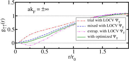
Figure 1: The trial, mixed and extrapolated $g_{\uparrow\uparrow}(r)$ with the LOCV $\Psi_{T}({\bf R})$ are compared with the trial $g_{\uparrow\uparrow}(r)$ with the $\Psi_{optim}({\bf R})$. Note that the mixed and trial pair distributions are the same for $\Psi_{optim}({\bf R})$. $r_{0}$ is given by $4\pi r_{0}^{3}\rho=3$.

This procedure assures that the nodes of $\Psi_{T}({\bf R})$ are near optimum, i.e. close to the nodes of the exact $\Psi_{0}({\bf R})$. However, the $\Psi_{T}({\bf R})$ itself can otherwise be very different from the $\Psi_{0}({\bf R})$. For example, in references Carlson et al. (2003) and Chang et al. (2004) we use

$$\Psi_{T}({\bf R})=\left[\prod\limits_{i,j^{\prime}}f_{\uparrow\downarrow}(r_{ij^{\prime}})\right]\Phi_{BCS}({\bf R})~{},$$ (5)

where $\Phi_{BCS}({\bf R})$ is a generalized Bardeen-Cooper-Schrieffer wave function, and its nodes are optimized by minimizing $\langle{\cal H}(\tau)\rangle_{mixed}$. The $f_{\uparrow\downarrow}(r_{ij^{\prime}})$ is a nodeless pair correlation function between spin up and down particles. The $\langle{\cal H}(\tau)\rangle_{mixed}$ does not depend upon the choice of $f_{\uparrow\downarrow}(r_{ij^{\prime}})$ in the limit $\tau\rightarrow\infty$. The $f_{\uparrow\downarrow}(r_{ij^{\prime}})$ is used to reach this limit quickly, and to reduce the variance of the stochastic evaluation of $\langle{\cal H}(\tau)\rangle_{mixed}$. Note that the commonly used Jastrow pair correlation function is also nodeless Feenberg (1969), but it acts between all pairs: $\uparrow\downarrow$, $\uparrow\uparrow$ and $\downarrow\downarrow$, and it is not useful in superfluid gases.

Mixed expectation values of other observables, $\langle{\cal O}\rangle_{mixed}$, can be easily calculated with GFMC, but they are more difficult to interprete when $[{\cal O},{\cal H}]\neq 0$. If one assumes that $|\Psi(\tau)\rangle=|\Psi_{T}\rangle+|\delta\Psi\rangle$, then the desired expectation value

$$\langle{\cal{O}}(\tau)\rangle = \frac{\langle\Psi(\tau)|{\cal O}|\Psi(\tau)\rangle}{\langle\Psi(\tau)|\Psi(\tau)\rangle}$$ (6)

$$= 2\langle{\cal{O}}(\tau)\rangle_{mixed}-\langle{\cal{O}}\rangle_{trial}$$

$$+\mbox{~{}terms of order }\delta\Psi^{2}~{}.$$

Here, the trial estimate $\langle{\cal{O}}\rangle_{trial}\equiv\langle\Psi_{T}|{\cal{O}}|\Psi_{T}\rangle/\langle\Psi_{T}|\Psi_{T}\rangle$. When $\delta\Psi$ is small, the extrapolation

$$\langle{\cal{O}}(\tau)\rangle_{extrap.}\approx 2\langle{\cal{O}}(\tau)\rangle_{mixed}-\langle{\cal{O}}\rangle_{trial}~{},$$ (7)

can be used to estimate $\langle{\cal O}\rangle$.

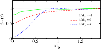
Figure 2: Optimized $f_{\uparrow\uparrow}(r)$ for different values of $ak_{F}$.

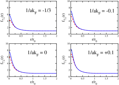
Figure 3: Optimized $f_{\uparrow\downarrow}(r)$ (dashed line) and LOCV $f_{\uparrow\downarrow}(r)$ (continuous line) for different values of $ak_{F}$.

However, in the strongly interacting regime the $\delta\Psi$ is not necessarily small, and this extrapolation may not be valid. For example, we consider the pair distribution function $g_{\uparrow\uparrow}(r)$ between parallel spin particles in the $ak_{F}\rightarrow\pm\infty$ limit. The mixed, trial and extrapolated values of $g_{\uparrow\uparrow}(r)$ obtained from the $\Psi_{T}({\bf R})$ of Ref. Carlson et al. (2003) and Chang et al. (2004) are shown in Fig. 1. At small $r$, the extrapolated $g_{\uparrow\uparrow}(r)<0$ indicating invalidity. These and all the other results presented in this work are obtained from Monte Carlo computations using 14 particles in a cubic periodic box. As discussed in Ref. Carlson et al. (2003) and Chang et al. (2004), a periodic box with 14 particles provides a fair approximation to the uniform gas. The cosh $v(r_{ij^{\prime}})$ with $\mu r_{0}=12$ is used Chang et al. (2004) to approximate the interaction between spin $\uparrow\downarrow$ pairs.

Table 1: Summary of the results in units of $E_{FG}$

$ak_{F}$	$\langle{\cal{H}}\rangle_{mixed}$	$\langle{\cal{H}}\rangle_{trial}$	$\langle{\cal{H}}\rangle_{optim}$	$\langle{\cal{V}}\rangle_{mixed}$	$\langle{\cal{V}}\rangle_{optim}$
-1	0.792(4)	0.818(3)	0.808(4)	-0.55(3)	-0.54(3)
-3	0.635(6)	0.85(3)	0.70(2)	-1.8(1)	-2.0(1)
-10	0.494(7)	0.68(3)	0.53(1)	-3.5(2)	-3.2(1)
$\infty$	0.414(5)	0.62(3)	0.46(1)	-3.9(1)	-4.0(2)
10	0.32(1)	0.57(6)	0.39(1)	-4.8(1)	-5.0(1)
3	-0.00(1)	0.4(1)	0.11(3)	-7.0(1)	-7.3(3)
2	-0.34(2)	0.2(1)	-0.18(3)	-9.2(4)	-9.2(3)
1	-2.37(3)	-0.1(1)	-2.01(3)	-19.0(4)	-18.0(6)

In principle, the pair correlation functions, $f_{\uparrow\downarrow}(r)$ and $f_{\uparrow\uparrow}(r)=f_{\downarrow\downarrow}(r)$ in $\Psi_{T}({\bf R})$ can be obtained by minimizing the trial energy $\langle{\cal H}\rangle_{trial}$. However, this variational problem has been approximately treated in most quantum Monte Carlo calculations. In Ref. Carlson et al. (2003); Chang et al. (2004) a simple and crude method called LOCV, based on constrained minimization of the leading two-body cluster contribution to $\langle{\cal H}\rangle_{trial}$ Schmidt et al. (1977) is used. In this method, $f_{\uparrow\uparrow}(r)=f_{\downarrow\downarrow}(r)=1$, and $f_{\uparrow\downarrow}(r)$ satisfies the two-body Schrödinger equation

$$-\frac{\hbar^{2}}{m}\nabla^{2}f_{\uparrow\downarrow}(r)+v(r)f_{\uparrow\downarrow}(r)=\lambda f_{\uparrow\downarrow}(r)~{},$$ (8)

at $r<d$. The boundary conditions are: $f_{\uparrow\downarrow}(r\geq d)=1$ and $f^{\prime}_{\uparrow\downarrow}(r=d)=0$. The healing distance $d$ serves as the variational parameter. The trial energies obtained with variational Monte Carlo (VMC) calculations using the optimum healing distance $d$ are compared with the FN-GFMC $\langle{\cal H}\rangle_{mixed}$ in Table 1. Both calculations use the optimum $\Phi_{BCS}({\bf R})$ found by minimizing the $\langle{\cal H}\rangle_{mixed}$ in Ref. Chang et al. (2004). The trial energies are well above $\langle{\cal H}\rangle_{mixed}$, particularly at $1/ak_{F}\geq 0$. This shows that the LOCV pair correlation functions are far from those in the exact $\Psi_{0}$ in the strongly interacting regime.

Here we present a new and simple method to optimize the pair correlation functions in the trial wave function using GFMC results. The optimized trial wave functions, denoted by $\Psi_{optim}({\bf R})$ are presumably close enough to $\Psi_{0}({\bf R})$ so that $\delta\Psi$ is small and Eq. 7 provides a fair approximation. The method can be improved and $\delta\Psi$ can be further decreased by including higher order correlations corresponding to triplet, quadruplet, etc. However, in the present work we consider only pair correlations for $\Psi_{optim}({\bf R})$ .

The trial pair distribution functions can be expressed as Feenberg (1969)

$$\langle g_{x}(r)\rangle_{trial}=f_{x}^{2}(r)~{}t_{x}(r,f_{\uparrow\uparrow},f_{\uparrow\downarrow},\Phi_{BCS}({\bf R}),\rho)~{},$$ (9)

where $x$ can be $\uparrow\uparrow$ or $\uparrow\downarrow$ and $t_{x}$ is a complicated function of $r$, $f_{\uparrow\uparrow},f_{\uparrow\downarrow}$, $\Phi_{BCS}({\bf R})$ and gas density $\rho$. It is difficult to calculate it exactly except by numerical methods. However, $t_{x}(r)$ contains many-body integrals, and is a relatively smooth function of $r$.

Our method to optimize $f_{x}(r)$ using GFMC is iterative. Let $\langle g_{x}^{(n)}(r)\rangle_{mixed}$ and $\langle g_{x}^{(n)}(r)\rangle_{trial}$ be obtained from the n-th trial $f_{x}^{(n)}(r)$ using the optimum $\Phi_{BCS}$ which does not depend on $f_{x}(r)$. We start with the LOCV approximation providing the $f_{x}^{(1)}(r)$, but one could start with any other choice of $f_{x}^{(1)}$ and converge to the same $\Psi_{optim}({\bf R})$ . The next improved $f_{x}^{(2)}(r)$ is chosen as

$$f_{x}^{(2)}(r)=f_{x}^{(1)}(r)\sqrt{\frac{\langle g_{x}^{(1)}(r)\rangle_{mixed}}{\langle g_{x}^{(1)}(r)\rangle_{trial}}}~{}.$$ (10)

If the difference between $f_{x}^{(1)}(r)$ and $f_{x}^{(2)}(r)$ is small, we can assume that the $t_{x}(r)$ functions do not change much. In this case $\langle g_{x}^{(2)}(r)\rangle_{trial}\approx\langle g_{x}^{(1)}(r)\rangle_{mixed}$. Otherwise, by iterating this process one easily converges to an $f_{x}^{(n)}(r)$ such that

$$\langle g_{x}^{(n)}(r)\rangle_{trial}\approx\langle g_{x}^{(n)}(r)\rangle_{mixed}~{}.$$ (11)

Usually, the convergence within statistical errors can be reached within 3 $\sim$ 4 iterations and it doesn’t seem to depend on the strength of the interaction. In practice, $\langle g_{x}(r)\rangle_{mixed}$ and $\langle g_{x}(r)\rangle_{trial}$ have Monte Carlo sampling errors. We approximate the square root of their ratio (Eq. 10) by a smooth function of $r$ chosen as $\cos(p_{1}r+p_{2})e^{-r/p_{3}}+1$, and vary the parameters $p_{1-3}$ to best fit the Monte Carlo values. One iteration step typically takes about 10 hours in a Pentium 3.0 GHz based workstation.

The VMC energies with the $\Psi_{optim}({\bf R})$ are much closer to the FN-GFMC energies (Table 1). In principle, the optimization of $f_{x}(r)$ should have no effect on the FN-GFMC $\langle{\cal H}\rangle_{mixed}$; in practice the $\langle{\cal H}\rangle_{mixed}$ seems to get lowered by $\sim 2\pm 1$ % after optimization presumably because the limit $\tau\rightarrow\infty$ is easier to reach with the $\Psi_{optim}({\bf R})$. The effects of the optimization are also seen in the reduced error bars of the energy estimates: $\delta\langle{\cal H}\rangle_{optim}\lesssim\delta\langle{\cal H}\rangle_{trial}$ (Table 1) for the same number of Monte Carlo samples. In addition, the $E_{T}$ (Eq. 2), which typically has larger fluctuations, becomes indistinguishable from $\langle{\cal H}\rangle_{mixed}$.

The pair distribution functions $\langle g_{x}(r)\rangle_{mixed}$ are determined by the many body probability distribution given by $\Psi_{optim}({\bf R})\Psi(\tau,{\bf R})$, while the $\langle g_{x}(r)\rangle_{optim}$ are for $|\Psi_{optim}({\bf R})|^{2}$. Note that $\Psi_{optim}({\bf R})\Psi(\tau,{\bf R})\approx\Psi_{optim}({\bf R})\Psi_{0}({\bf R})\geq 0$ since the nodes of $\Psi_{optim}({\bf R})$ have been varied to match those of $\Psi_{0}({\bf R})$.

Extending the above method, if we can match the mixed and optimized trial distributions for all, pair, triplet, quadruplet, $\dots$ distribution functions, then we can assume that $\Psi_{optim}({\bf R})=\Psi_{0}({\bf R})$. However, here we approximate the exact $\Psi_{0}({\bf R})$ by $\Psi_{optim}({\bf R})$ using $\Phi_{BCS}({\bf R})$ and pair correlation functions only

$$\Psi_{optim}({\bf R}) = \prod\limits_{i,j^{\prime}}f_{\uparrow\downarrow}^{optim}(r_{ij^{\prime}})\prod\limits_{i<j}f_{\uparrow\uparrow}^{optim}(r_{ij})$$ (12)

$$\times\prod\limits_{i^{\prime}<j^{\prime}}f_{\downarrow\downarrow}^{optim}(r_{i^{\prime}j^{\prime}})\Phi_{BCS}({\bf R})~{}.$$

The validity of Eq. 11 ensures that the present optimization method will converge to $f_{x}^{(n)}\rightarrow f_{x}^{optim}(r)$ and thus $\Psi_{optim}({\bf R})$ is as close to $\Psi_{0}({\bf R})$ as its form (Eq. 12) allows. If higher order correlations have negligible effects on the wave functuion, we should expect

$$\langle{\cal H}\rangle_{optim}\approx\langle{\cal H}\rangle_{mixed}\approx E_{0}~{}.$$ (13)

However, in the interesting regime of $ak_{F}\sim\infty$, Table 1 shows that the $\langle{\cal H}\rangle_{optim}$ is larger than the $\langle{\cal H}\rangle_{mixed}$ by $\sim$ 10 %. This suggests that the form of the present $\Psi_{optim}({\bf R})$ is not sufficiently general. An improved approximation could be obtained by including products of triplet correlations $F_{P}(r_{ij},r_{jk},r_{ki})$ for $\uparrow\uparrow\uparrow$ and $\downarrow\downarrow\downarrow$, and $F_{M}(r_{ij},r_{jk^{\prime}},r_{k^{\prime}i})$ for $\uparrow\uparrow\downarrow$ and $\downarrow\downarrow\uparrow$ triplets in the wave function. We believe that the present method can be generalize to determine the optimal forms of three-body correlations by making

$$g_{3,x}(r_{ij},r_{jk},r_{ki})_{mixed}=g_{3,x}(r_{ij},r_{jk},r_{ki})_{optim}~{},$$ (14)

where $g_{3}$ denotes three particle distribution functions. The true $\Psi_{0}$ can also have backflow correlations Schmidt et al. (1981); however, they change the nodal surface and have to be optimized by minimizing $\langle{\cal H}\rangle_{mixed}$.

The main difference between the optimum pair correlations and those of Ref. Carlson et al. (2003) and Chang et al. (2004) is in $f_{\uparrow\uparrow}(r)$. In LOCV we have $f_{\uparrow\uparrow}(r)=1$, because in two-body clusters there is no interaction between parallel spin particles in dilute Fermi gases. However, many body effects generate an effective repulsion between parallel spin particles and the optimum $f_{\uparrow\uparrow}(r)$ is $<1$ at $r\lesssim 1.5r_{0}$ as shown in Fig. 2.

The optimum and LOCV $f_{\uparrow\downarrow}(r)$ are generated by the strong two body attraction in $\uparrow\downarrow$ pairs and have qualitatively similar shapes (Fig. 3). For $1/ak_{F}<<-1$, the LOCV $f_{\uparrow\downarrow}(r)$ is near optimum. For stronger interactions, it is larger than the optimum at $r\sim 0$ (Fig. 3).

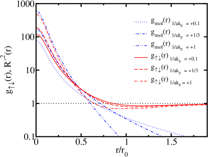
Figure 4: Comparison of the pair distribution function $g_{\uparrow\downarrow}(r)$ with the radial probability distribution of the molecule in the $a>0$ regime.

The expectation value of the potential energy, $\langle{\cal V}\rangle=\langle\sum_{i,j^{\prime}}v(r_{ij^{\prime}})\rangle$ can easily be calculated from the GFMC (mixed) and VMC distributions using $\Psi_{optim}$. The calculated values of the potential energy are given in the last two columns of Table 1. Apart from statistical fluctuations, the mixed and the optimum pair distribution functions are the same. Therefore no extrapolation, such as in Eq. 7, is necessary for calculating $\langle{\cal V}\rangle$ using $\Psi_{optim}({\bf R})$.

Only when $1/ak_{F}>0$, we can have bound states with normalized radial wave functions $R(r)$. We define $R^{\prime}(r)=\sqrt{\frac{2}{\rho}}R(r)$ so that $g_{mol}(r_{\uparrow\downarrow})\equiv R^{\prime 2}(r)$ is normalized analogous to $g_{\uparrow\downarrow}(r)$, and the two are compared in Fig. 4 ($g_{\uparrow\downarrow}(r)$ is normalized such that $g_{\uparrow\downarrow}(r)\rightarrow 1$ for $r\rightarrow\infty$). When $1/ak_{F}\rightarrow 0^{+}$, we know that $g_{mol}(r)=R^{\prime 2}(r)\rightarrow 0$ (infinite pair size), but $g_{\uparrow\downarrow}(r)\gtrsim 1$. So $g_{mol}(r)$ and $g_{\uparrow\downarrow}(r)$ are qualitatively different when $a$ is large. However, when the interaction is stronger and $a$ becomes positive and small we expect a gas of molecules in which $g_{\uparrow\downarrow}(r)\sim g_{mol}(r)$ at $r<$ the size of the molecule. Fig. 4 shows that the superfluid may well be approximated by a gas of molecules with BEC for $1/ak_{F}\gtrsim 1/3$. The molecule size for $1/ak_{F}=1/3$, is $1.21r_{0}$ and for $1/ak_{F}=1$, it is $0.38r_{0}$. Due to the many body effects in $g_{\uparrow\downarrow}(r)$, it is meaningless to compare beyond these distances. In fact, for all $ak_{F}>0$, the $g_{mol}(r)\rightarrow 0$ while $g_{\uparrow\downarrow}(r)\rightarrow 1$ as $r\rightarrow\infty$.

In conclusion, the proposed method allows us to optimize separately the BCS and the pair correlations in dilute Fermi gases. The BCS and $f_{\uparrow\downarrow}(r)$ correlations are most important, however in the strong interaction regime, the $f_{\uparrow\uparrow}(r)$ can not be neglected.

The studies of momentum distributions and density matrices of the superfluid gas may now be possible using the optimum $\Psi_{T}({\bf R})$, and are in progress.

This work is partly supported by the U.S. National Science Foundation via grant PHY-03-55014.

References

De Marco et al. (1999)
B. De Marco,
and
D. S. Jin,
Science
285, 1703 (1999).
O’Hara et al. (2002)
K. M. O’Hara,
S. L. Hemmer,
M. E. Gehm,
S. R. Granade,
and J. E.
Thomas, Science
298, 2179 (2002).
Roberts et al. (2001)
J. L. Roberts,
N. R. Claussen,
S. L. Cornish,
E. A. Donley,
E. A. Cornell,
and C. E.
Wieman, Phys. Rev. Lett.
86, 4211 (2001).
Regal et al. (2003)
C. A. Regal,
C. Ticknor,
J. L. Bohn, and
D. S. Jin,
Nature 424,
47 (2003).
Regal et al. (2004)
C. A. Regal,
M. Greiner, and
D. S. Jin,
Phys. Rev. Lett. 92,
040403 (2004).
Bartenstein et al. (2003)
M. Bartenstein,
A. Altmeyer,
S. Riedl,
S. Jochim,
C. Chin,
J. H. Denschlag,
and
R. Grimm,
Phys. Rev. Lett. 92,
120401-1 (2004).
Randeria (1995)
M. Randeria, in
Bose-Einstein Condensation, edited by
A. Griffin,
D. Snoke, and
S. Stringari
(Cambridge, 1995).
Carlson et al. (2003)
J. Carlson,
S. Y. Chang,
V. R. Pandharipande,
and
K. E. Schmidt,
Phys. Rev. Lett. 91,
50401 (2003).
Chang et al. (2004)
S. Y. Chang,
V. R. Pandharipande,
J. Carlson,
and
K. E. Schmidt,
Phys. Rev. A 70,
043602 (2004).
Astrakharchik et al. (2004)
G. E. Astrakharchik,
J. Boronat,
J. Casulleras,
and
S. Giorgini,
Phys. Rev. Lett. 93,
200404
(2004).
Pethick et al (1995)
C. J. Pethick,
and
D. G. Ravenhall,
Ann. Rev. Nuc. Part. Scince 45,
429 (1995).
Dean et al (2003)
D. J. Dean,
and
M. Hjorth-Jensen,
Rev. Mod. Phys. 75,
607 (2003).
Anderson (1975)
J. B. Anderson,
J. Chem. Phys. 63,
1499 (1975).
Kalos (1974)
M. H. Kalos,
D. Levesque,
and
L. Verlet,
Phys. Rev. A 9,
2178 (1974).
Feenberg (1969)
E. Feenberg,
Theory of quantum fluids,
(Academic Press, 1969).
Schmidt et al. (1977)
V. R. Pandharipande,
and K. E.
Schmidt,
Phys. Rev. A 15,
2486 (1977).
Schmidt et al. (1981)
K. E. Schmidt,
M. A. Lee,
M. H. Kalos, and
G. V. Chester,
Phys. Rev. Lett. 47,
807 (1981).