A Simple Model of Scale-free Networks
Driven by Both Randomness and Adaptability

Abstract

In this paper, we present a simple model of scale-free networks that incorporates both preferential & random attachment and anti-preferential & random deletion at each time step. We derive the degree distribution analytically and show that it follows a power law with the degree exponent in the range of $(2,\infty)$. We also find a way to derive an expression of the clustering coefficient for growing networks and compute the average path length through simulation.

PACS: 84.35.+i; 64.60.Fr; 87.23.Ge

Keywords: scale-free network, degree distribution, clustering coefficient, average path length

Dinghua Shi¹ ,  Xiang Zhu²  and  Liming Liu ^2,

¹Department of Mathematics, College of Science, Shanghai University,

Shanghai 200436, China

E-mail address: shidh2001@263.net

²Department of Industrial Engineering and Engineering Management,

Hong Kong University of Science and Technology,

Clear Water Bay, Kowloon, Hong Kong

E-mail address: zhuxiang@ust.hk

1 Introduction

Complex networks play a crucial role in a wide range of practical systems of technological, biological, and social importance [1, 2]. For example, the Internet, the World Wide Web (WWW), communities of scientists and biological cells can all be described as complex networks. Although various complex networks exist in various different fields, their evolutions are driven by a few rules. We believe that three intrinsic rules are behind the evolutions of most complex networks. They are randomness, adaptability and hereditary. The existing investigations usually focus on one or two of the three rules.

The earliest study of complex networks can be traced to the investigation of regular graphs characterized by a large clustering coefficient and a long average path length. Erdös and Rényi [3] initiate the studies of complex networks as random graphs. They propose the ER model which has a short average path length and a small clustering coefficient. Later observations have found that some real networks have not only short average path lengths like random graphs but also large clustering coefficients like regular graphs. These two features characterize the small-world network. Watts and Strogats [4] later develop a model based on regular graphs in which links are random rewired with a fixed probability. For some range of small rewiring probabilities, their model successfully displays the small-world characteristics. Two things are common for random graphs and small-world networks: randomness of connections between nodes and exponential decay of the tail of the degree distribution.

However, more recent empirical evidences from the Internet and WWW, among other complex networks, show a fundamentally different picture, i.e., the tail of the degree distribution follows a power law. Two general features have been observed in many real-world networks: successive additions of new nodes and preference to link to the existing nodes. This shows that randomness is not the unique feature of networks and leads to the introduction of scale-free networks in 1999 by Albert, Baraba$\acute{a}$si, and Jeong in their pioneering works [5, 6, 7], which start a new phase in the study of complex networks. Albert, Baraba$\acute{a}$si, and Jeong propose two mechanisms to characterize the evolution of a scale-free network [6, 7]: the growth, starting from $m_{0}$ nodes, the network grows at a constant speed, i.e., adding one node at each time step and connecting to $m~{}(m\leq m_{0})$ existing nodes; the preferential attachment, the chance that an existing node receives a connection from a new node is proportional to the number of connections it already has. Here the phenomenon of preferential attachment reflects the adaptability of complex network. The authors show that, under these two mechanisms, a network evolves into a stationary scale-free state. Its degree distribution follows a power law with the degree exponent $\gamma=2.9\pm 0.1$ from simulation analysis and $\gamma=3$ from the analytical result. These results are significant for complex networks and these two mechanisms become the first model, referred to as the BA model. Although the BA model can be used to interpret many phenomena of complex networks, the degree exponent is a constant, which is a weakness since most empirical studies shows that $\gamma$ can be either less than $3$ or large than $3$ in real complex networks [1].

To improve the original BA model, many researchers suggest different mechanisms for both growth and preferential attachment under which the range of $\gamma$ varies from $2$ to infinity. In the following, we will briefly review some significant works.

Krapivsky, Redner, Leyvraz [8] examine the effect of a nonlinear preferential connection probability $\Pi(k)$ on complex networks. By analyzing the rate equation, they demonstrate that the topology of the network is scale-free only when the preferential attachment is asymptotically linear. Dorogovtsev, Mendes, and Samukhin [9] use a master-equation approach to study complex networks in which the probability $\Pi(k)$ is proportional to the sum of a node’s initial attractiveness and the number of incoming edges. By applying mean-field theory, Dorogovtsev and Mends [10] consider both preferential attachment and random removal (with equal probability) in the evolution of a network. Albert, Baraba$\acute{a}$si [11] study internal edges and rewiring, Dorogovtsev and Mends [12] propose models for gradual aging.

Different from the BA model, Krapivsky, Rodgers, Render [13] consider a growing network with directed edges. In their model, at each time step, either a new node or a new link is randomly added to the network and the attachment probability depends on the in- or out-degrees of nodes. By solving rate equations, they conclude that both in- and out-degree exponents lies in $(2,\infty)$. Kleinberg et al. [14], Kumar et al. [15, 16] address an alternative preferential mechanism named copy mechanism by adding random links with “prototype” nodes. It is found that the copy mechanism is equivalent to a linear preferential attachment. Krapivsky and Render [17]’s edge redirection mechanisms is mathematically equivalent to Kumar et al.’s model discussed above.

From the reviewed works, we find two common facts: (1) under linear growth, the range of the degree exponent can be extended to infinity by adding randomness into model; (2) local events and growth constraints have a similar function, which is to make the degree exponent vary between $2$ and $3$. Although the above research extends the range of the degree exponent, their proposed mechanisms are relatively complex. Compared with the above models, Liu et. al [18]’s model is relatively simple. It combines the ideas from [3] and [6] to model the probability that a new node is connected to node $i$ already in the network. They find that the degree exponent is no less than $3$, so the model is not applicable to situations when the degree exponent is between $2$ and $3$, which is the most common range observed in real world. Recently, Chen and Shi [19] introduces the concept of anti-preferential deletion into the BA model and show that $2<\gamma<3$. This shows that integrating randomness and anti-preferential deletion into the BA model, one may construct a simple model for a general class of scale-free networks with $\gamma>2$.

This research is mainly motivated by the above observation. Based on [18] and [19], we propose a simple evolution model of complex networks with preferential and random attachment, anti-preferential and random deletion. We show that the network self-organizes into a scale-free network. We obtain  the expression of the degree exponent analytically, and find it lies in $(2,\infty)$. Clustering coefficient is another key network parameter, but analytical estimations are hard to obtain for growth networks as reflected by the current state of the literature. In this paper, we are able to derive an analytical expression for the clustering coefficient. Our method can be useful for similar studies. In short, our model is constructed from simple mechanisms and can be applied to analyze a general class of complex networks.

We organize the paper as follows. In the next section, we present a simple model of scale-free network. In section 3, we obtain the degree exponent analytically. Section 4 develops a method to derive the clustering coefficient. Section 5 discusses the average path length. We conclude the paper in Section 6 by pointing out some future research opportunities.

2 Model Description

Our network starts with $m_{0}$ completely connected nodes. At each time step, the following two procedures are performed:

(i) A new node is added to the system: $m(\leq m_{0})$ new edges from the new node are connected to $m$ different existing nodes. A node $i$ with degree $k_{i}$ will receive a connection from the new node with the linear-preferential probability

$$\Pi(k_{i})=\frac{(1-p)k_{i}+p}{\sum_{j}[(1-p)k_{j}+p]},$$ (1)

where $p$ is the probability that the selection of an existing node (for attachment) is random while $(1-p)$ is the probability that the selection of an existing node (for attachment) preferential.

(ii) $c$ old links are deleted: We first select node $i$ with at least one link as one end of a link with the anti-linear-preferential probability

$$\Pi^{*}(k_{i})=N^{-1}(t-1)[1-\Pi(k_{i})],$$ (2)

where $N(t-1)$ is the number of connected nodes with nonempty links at $t$ time step and $N^{-1}(t-1)$ is used as the normalized coefficient such that $\sum_{i}\Pi^{*}(k_{i})=1.$ Then, we choose another node $j$ from the neighborhood of node $i$ (denoted as $O_{i}$ ) as the other end of the link with probability $K_{i}^{-1}\Pi^{*}(k_{j})$, where $K_{i}=\sum_{j\in O_{i}}\Pi^{*}(k_{j})$. We delete the link connecting nodes $i$ and $j$. We repeat this procedure $c$ times to delete $c$ old links.

The basic ideas of the above process is to use a linear combination of a random selection probability and a preferential selection probability as the selection probability. We believe that this linear selection rule for attachment and deletion models real world networks more closely, from the point of view of the evolutionary theory.

3 Degree Distribution

By the continuum theory, $k_{i}(t)$ approximately satisfies the following dynamic equation:

$$\frac{\partial k_{i}}{\partial t} = m\Pi(k_{i})-c\left[\Pi^{*}(k_{i})+\sum_{j\in O_{i}}\Pi^{*}(k_{j})K_{j}^{-1}\Pi^{*}(k_{i})\right]$$ (3)

$$= m\Pi(k_{i})-c\left[\Pi^{*}(k_{i})+\Pi^{*}(k_{i})\sum_{j\in O_{i}}K_{j}^{-1}\Pi^{*}(k_{j})\right]$$

$$\approx m\frac{(1-p)k_{i}+p}{[2(1-p)(m-c)+p]t}-c\frac{2}{t},~{}~{}~{}\mbox{for large $t$}\hskip 2.84544pt$$

where the last approximation comes from $\sum_{j}[(1-p)k_{j}+p]=[2(1-p)(m-c)+p]t$ and $\{\Pi^{*}(k_{i})+\Pi^{*}(k_{i})\sum_{j\in O_{i}}K_{j}^{-1}\Pi^{*}(k_{j})\}\approx 2/t$. In the approximation, we assume that $N(t-1)\approx t$ and $\sum_{j\in O_{i}}K_{j}^{-1}\Pi^{*}(k_{j})\approx 1$. Near the end of next session, we give a simulation result to check the accuracy of degree exponent obtained under this assumption.

Let $t_{i}$ be the time step when node $i$ is added to the network. Initially, node $i$ has $k_{i}(t_{i})=m$ links, thus the above equation has the following solution:

$$k_{i}(t)=B\left[\left(\frac{t}{t_{i}}\right)^{\beta}-1\right]+m,\hskip 2.84544pt\mbox{for large $t$}$$ (4)

where the dynamic exponent

$$\beta=\beta(m,p,c)=\frac{m(1-p)}{2(1-p)(m-c)+p},$$ (5)

and the coefficient

$$B=B(m,p,c)=m+\frac{mp-2c[2(1-p)(m-c)+p]}{m(1-p)}.$$ (6)

In the solution procedure, we require $0<\beta<1$ and $B>0$ for the feasible solution. To guarantee $0<\beta<1$, the parameters should satisfy

$$(1-p)(m-2c)+p>0.$$ (7)

On the other hand, the condition $B>0$ holds if and only if

$$m^{2}(1-p)+mp-4c(1-p)(m-c)-2cp > 0\Leftrightarrow$$

$$(1-p)(m-2c)^{2}+p(m-2c) > 0\Leftrightarrow$$

$$(m-2c)[(1-p)(m-2c)+p] > 0.$$

Therefore, we conclude that $B>0$ if only if (7) is held. In sum, we see that $m>2c$ is a sufficient condition for both $0<\beta<1$ and $B>0$.

Assume that $t_{i}$ follows the uniform distribution over interval $(0,t)$. Then, by (4), we have

$$P(k_{i}(t)<k) = 1-(\frac{B}{B-m+k})^{1/\beta}\frac{t}{m_{0}+t},$$

$$P(k,t) = \frac{\partial P(k_{i}(t)<k)}{\partial k}$$

$$= \frac{t}{m_{0}+t}\frac{1}{\beta}B^{1/\beta}(k+B-m)^{-\gamma},$$

$$P(k) = \frac{1}{\beta}B^{1/\beta}(k+B-m)^{-\gamma},~{}~{}~{}(t\rightarrow\infty),$$ (8)

where

$$\gamma=1+\frac{1}{\beta}=3+\frac{p-2c(1-p)}{m(1-p)}.$$ (9)

Thus, this system self-organizes into a scale-free network with a degree exponent given by (9).

Since $[p-2c(1-p)]/[m(1-p)]$ is increasing in $p$ and $\gamma=3-2c/m>2$ for $p=0$, we have $\gamma>2$. In particular, when $p\leq 2c(1-p)$, we can generate values of $\gamma$ between $2$ and $3$. Such $\gamma$ values have been observed in different networks including the WWW and movie actor collaboration networks [7]. For $p\rightarrow 1$, we have $\gamma\rightarrow\infty$ while for $(1-p)(m-2c)+p\rightarrow 0$, we obtain $\gamma\rightarrow 2$. Further, when $p=c=0$, it yields the BA model [6]; when $p=0$ and $c>0$, it gives Model B (with $n=0$) proposed by Chen and Shi [19]; when $p>0$ and $c=0$, it is equivalent to the model studied in Liu et. al [18].

We now use simulation to compute the degree distribution of our model. We set $m_{0}=10$, $m=5$, $c=1$ and $p=0.667$. Analytically, $\gamma=3$ from (9). In the experiment, we take the average from $100$ runs. After computation, we obtain $\gamma\approx 2.996$, and the coefficient is $29.692$. Figure 1 shows that the results of the simulation, which indicates the approximations in (3) are reasonable.

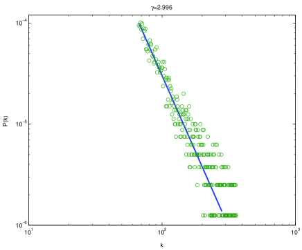
Figure 1: the Degree Distribution

Remark 1.

Suppose that at each time step, we also perform an additional process: $n$ new edges between old nodes are produced: a node $i$ is selected as a end of a new edge, with the probability $\Pi(k_{i})$ given by (1). Then, the new degree exponent is given by

$$\gamma=3+\frac{p-2(1-p)(n+c)}{(m+2n)(1-p)}.$$ (10)

We can show that this process has no impact on the range of $\gamma$. Further, by (10), when we let $c=0$, we find that the range of $\gamma$ is kept the same under the effect of $n$, which indicates that the function of adding new edges between old nodes is equivalent to that of anti-linear-preferential deletion.

Remark 2.

Now, at each time step, we consider another additional operation: we rewire $n$ existing edges in the network: select randomly a node $i$ and a link $l_{ij}$ connected to it. Next we rewire this link and replace it with a new link $l_{i^{\prime}j}$ that connects node $j$ and node $i^{\prime}$ chosen with the probability $\Pi(k_{i})$ given by (1). This operation is repeated $n$ times. As a result, the degree exponent is given by

$$\gamma=3+\frac{p-2(1-p)(n+c)}{(m+n)(1-p)}.$$ (11)

Clearly, $n$ also does not affect the range of $\gamma$. Moreover, if we let $c=0$, we see that the function of rewiring old edges between old nodes is equivalent to that of anti-linear-preferential deletion.

4 Clustering Coefficient

In this section, we present a method to derive an explicit expression for clustering coefficients of growing network models.

Consider a node $l$. When the size of the network is $N$, there will be $k_{l}(N)$ nodes in its neighborhood. The maximum possible number of links among all the neighbors of node $l$ is $k_{l}(N)[k_{l}(N)-1]/2$. The clustering coefficient $C_{l}(N)$ of node $l$ is then defined as the ratio between the actual number of links among all the nodes in the neighborhood and $k_{l}(N)[k_{l}(N)-1]/2$. The clustering coefficient of the network is then the average of the clustering coefficients of all the nodes in the network.

To compute the clustering coefficient, we will rewrite dynamic equation (3) in the following integral form

$$k_{i}(t)=m+\int_{i}^{t}\frac{m(1-p)k_{i}(j)+mp-2ca_{1}}{a_{1}j}dj,$$ (12)

where $a_{1}=2(1-p)(m-c)+p>0$.

From (12), we find that the expected number of links connecting node $i$ added at the $i$th time step with node $j$ added at the $j$th time epoch up to time step $t$ is given by

$$\int_{i}^{t}\frac{m(1-p)k_{i}(j)+mp-2ca_{1}}{a_{1}j}dj.$$

Next, by continuous theory, we obtain that the probability for the existence of a link from the node $j$ to node $i$ ($i<j$), i.e.,

$$Prob\{(ij)\} = \frac{m(1-p)k_{i}(j)+mp-2ca_{1}}{a_{1}j}$$ (13)

$$= \frac{a_{2}j^{\beta-1}}{a_{1}i^{\beta}},$$

where the second equality is followed from (4) and $a_{2}=m^{2}(1-p)+mp-2ca_{1}>0$.

To find the number of actual connections among neighbors of a given node $l$, we need to consider the sequence (age) by which node $l$ and its neighbors appear. For example, $l<i<j$ means that node $l$ is older than node $i$ which is in turn older than node $j$. Then, the expected number of edges between node $i$ and node $j$ that are neighbors of node $l$ is given by $\int_{l}^{N}dip(li)\int_{i}^{N}djp(lj)p(ij).$ Similarly, we have to count five other cases: $i<l<j$, $i<j<l$, $l<j<i$, $j<l<i$ and $j<i<l$. The related integration expressions of six cases are given in (14), respectively. Note that we count the links between any two node twice, we need to divide the sum of six integrations by $2$. Also, we approximate the maximum number of connections by $k_{l}(N)^{2}/2$. Thus, we obtain

$$C_{l}(N) = \frac{1}{k_{l}(N)^{2}}\left[\int_{l}^{N}dip(li)\int_{i}^{N}djp(lj)p(ij)+\int_{1}^{l}dip(il)\int_{l}^{N}djp(lj)p(ij)\right.$$ (14)

$$\left.+\int_{1}^{l}dip(il)\int_{i}^{l}djp(jl)p(ij)+\int_{l}^{N}dip(li)\int_{l}^{i}djp(lj)p(ji)\right.$$

$$\left.+\int_{l}^{N}dip(li)\int_{1}^{l}djp(jl)p(ji)+\int_{1}^{l}dip(il)\int_{1}^{i}djp(jl)p(ji)\right].$$

Now, we consider first two extreme cases of our model: $\beta=0.5$ and $\beta=0$. For $\beta=0.5$, we set $p=0$, $c=0$. In this case, our model is equivalent to the BA model, and $p(ij)=p(ji)=m(ij)^{-1/2}/2$. Furthermore, (14) can be simplified to

$$C_{l}(N) = \frac{\int_{1}^{N}dip(li)\int_{1}^{N}djp(lj)p(ij)}{k_{l}(N)^{2}}$$ (15)

$$= m(\ln N)^{2}/(8N)$$

$$\propto \frac{(\ln N)^{2}}{N}.$$

The last equation is the same as the one provided in [23]. Noting that $C_{l}(N)$ is independent of $l$, (15) also gives the cluster coefficient of the whole network.

When $c=0$ and $p=1$, $\beta=0$ and we have a random network. We can rewrite (13) as

$$Prob\{(ij)\} = \frac{m}{j}.$$ (16)

The integrations of (14) can be simplified,

$$\int_{l}^{N}dip(li)\int_{i}^{N}djp(lj)p(ij) = \int_{l}^{N}dip(li)\int_{l}^{i}djp(lj)p(ji)=m^{3}(l^{-1}-N^{-1}-\frac{\ln N-\ln l}{N}),$$

$$\int_{1}^{l}dip(il)\int_{l}^{N}djp(lj)p(ij) = \int_{l}^{N}dip(li)\int_{1}^{l}djp(jl)p(ji)=m^{3}\frac{l-1}{l}(l^{-1}-N^{-1}),$$

$$\int_{1}^{l}dip(il)\int_{i}^{l}djp(jl)p(ij) = \int_{1}^{l}dip(il)\int_{1}^{i}djp(jl)p(ji)=m^{3}\frac{l-1-\ln l}{l^{2}}.$$

Using $k_{l}(N)\approx m\ln N$ as in [18], we can similarly obtain

$$C_{l}(N) = m\left[l^{-1}-N^{-1}-\frac{\ln N-\ln l}{N}+\frac{l-1}{l}(l^{-1}-N^{-1})+\frac{l-1-\ln l}{l^{2}}\right]/(\ln N)^{2},$$

$$= m\left[2(l^{-1}-N^{-1})-\frac{\ln N-\ln l}{N}-\frac{l^{-1}-N^{-1}}{l}+\frac{l-1-\ln l}{l^{2}}\right]/(\ln N)^{2}.$$

It is easy to see that

$$C(N) = \int_{1}^{N}C_{l}(N)dl/N\propto\frac{1}{N\ln N}.$$ (17)

The analytical results obtained above for random networks are new.

For the general case, explicit formula for the clustering coefficient is more difficult to obtain. The following analysis provides a good general approximation.

We need to compute the $6$ integrations in (14) separately. For $l<i<j$, we have

$$\int_{l}^{N}dip(li)\int_{i}^{N}djp(lj)p(ij) = \int_{l}^{N}\frac{a_{2}i^{\beta-1}}{a_{1}l^{\beta}}di\int_{i}^{N}\frac{a_{2}j^{\beta-1}}{a_{1}l^{\beta}}\times\frac{a_{2}j^{\beta-1}}{a_{1}i^{\beta}}dj$$

$$= \frac{a_{2}^{3}l^{-2\beta}}{a_{1}^{3}}\left[\frac{N^{2\beta-1}(\ln N-\ln l)}{2\beta-1}-\frac{N^{2\beta-1}-l^{2\beta-1}}{(2\beta-1)^{2}}\right].$$

For $i<l<j$,

$$\int_{1}^{l}dip(il)\int_{l}^{N}djp(lj)p(ij) = \int_{1}^{l}\frac{a_{2}l^{\beta-1}}{a_{1}i^{\beta}}di\int_{l}^{N}\frac{a_{2}j^{\beta-1}}{a_{1}l^{\beta}}\times\frac{a_{2}j^{\beta-1}}{a_{1}i^{\beta}}dj$$

$$= \frac{a_{2}^{3}l^{-1}}{a_{1}^{3}}\frac{(1-l^{-2\beta+1})N^{2\beta-1}-l^{2\beta-1}+1}{(2\beta-1)^{2}}.$$

For $i<j<l$,

$$\int_{1}^{l}dip(il)\int_{i}^{l}djp(jl)p(ij) = \int_{1}^{l}\frac{a_{2}(l/i)^{\beta}}{a_{1}l}di\int_{i}^{l}\frac{a_{2}(l/j)^{\beta}}{a_{1}l}\times\frac{a_{2}(j/i)^{\beta}}{a_{1}j}dj$$

$$= \frac{a_{2}^{3}l^{2\beta-2}}{a_{1}^{3}}\left[\frac{\ln l}{2\beta-1}+\frac{l^{-2\beta+1}-1}{(2\beta-1)^{2}}\right].$$

For $l<j<i$,

$$\int_{l}^{N}dip(li)\int_{l}^{i}djp(lj)p(ji) = \int_{l}^{N}\frac{a_{2}i^{\beta-1}}{a_{1}l^{\beta}}di\int_{l}^{i}\frac{a_{2}j^{\beta-1}}{a_{1}l^{\beta}}\times\frac{a_{2}i^{\beta-1}}{a_{1}j^{\beta}}dj$$

$$= \frac{a_{2}^{3}l^{-2\beta}}{a_{1}^{3}}\left[\frac{N^{2\beta-1}(\ln N-\ln l)}{2\beta-1}-\frac{N^{2\beta-1}-l^{2\beta-1}}{(2\beta-1)^{2}}\right].$$

For $j<l<i$,

$$\int_{l}^{N}dip(li)\int_{1}^{l}djp(jl)p(ji) = \int_{l}^{N}\frac{a_{2}i^{\beta-1}}{a_{1}l^{\beta}}di\int_{1}^{l}\frac{a_{2}l^{\beta-1}}{a_{1}j^{\beta}}\times\frac{a_{2}i^{\beta-1}}{a_{1}j^{\beta}}dj$$

$$= \frac{a_{2}^{3}l^{-1}}{a_{1}^{3}}\frac{(1-l^{-2\beta+1})N^{2\beta-1}-l^{2\beta-1}+1}{(2\beta-1)^{2}}.$$

For $j<i<l$,

$$\int_{1}^{l}dip(il)\int_{1}^{i}djp(jl)p(ji) = \int_{1}^{l}\frac{a_{2}l^{\beta-1}}{a_{1}i^{\beta}}di\int_{1}^{i}\frac{a_{2}l^{\beta-1}}{a_{1}j^{\beta}}\times\frac{a_{2}i^{\beta-1}}{a_{1}j^{\beta}}dj$$

$$= \frac{a_{2}^{3}l^{2\beta-2}}{a_{1}^{3}}\left[\frac{\ln l}{2\beta-1}+\frac{l^{-2\beta+1}-1}{(2\beta-1)^{2}}\right].$$

Putting the summation together, we obtain the expectation number of actual connections among neighbors of a given node $l$:

$$E = (\frac{a_{2}}{a_{1}})^{3}\left\{\frac{N^{2\beta-1}[l^{-2\beta}(2\beta-1)(\ln N-\ln l)-2l^{-2\beta}+l^{-1}]}{(2\beta-1)^{2}}\right.$$ (18)

$$\left.+\frac{l^{2\beta-2}(2\beta-1)\ln l+3l^{-1}-2l^{2\beta-2}}{(2\beta-1)^{2}}\right\}.$$

Substituting (18) and $k_{l}(N)^{2}$, noting (4), into (14), we obtain

$$C_{l}(N) = 2(\frac{a_{2}}{a_{1}})^{3}\left\{\frac{N^{2\beta-1}[(2\beta-1)(\ln N-\ln l)-2+l^{2\beta-1}]}{(2\beta-1)^{2}[BN^{\beta}-(B-m)l^{\beta}]^{2}}\right.$$ (19)

$$\left.+\frac{l^{4\beta-2}(2\beta-1)\ln l+3l^{2\beta-1}-2l^{4\beta-2}}{(2\beta-1)^{2}[BN^{\beta}-(B-m)l^{\beta}]^{2}}\right\}.$$

Analytical integration of the above equation is next to impossible in general. For an approximation of the network clustering coefficient and to identify it asymptotic behavior as $N$ becomes large, it is reasonable to approximate $k_{l}(N)$ by $B(N/l)^{\beta}$. This allows us to rewrite (19) as

$$C_{l}(N) \approx 2(\frac{a_{2}}{a_{1}})^{3}\frac{N^{2\beta-1}[(2\beta-1)(\ln N-\ln l)-2}{B^{2}(2\beta-1)^{2}N^{2\beta}}$$ (20)

$$+\frac{l^{2\beta-1}]+l^{4\beta-2}(2\beta-1)\ln l+3l^{2\beta-1}-2l^{4\beta-2}}{B^{2}(2\beta-1)^{2}N^{2\beta}}.$$

Taking average on both sides of (20), it is easy to conclude that

$$C(N) = \int_{1}^{N}C_{l}(N)dl/N$$ (21)

$$\propto \frac{N^{-2\beta-1}}{B^{2}(2\beta-1)^{2}}\left\{N^{4\beta-1}[\frac{1}{2\beta}+\frac{2\beta-1}{4\beta-1}\ln N-\frac{2\beta-1}{(4\beta-1)^{2}}-\frac{2}{4\beta-1}]\right.$$

$$+N^{2\beta}(2\beta-3+\frac{3}{2\beta})-N^{2\beta-1}(2\beta-3+(2\beta-1)\ln N+\frac{1}{2\beta})$$

$$\left.+\frac{2\beta-1}{(4\beta-1)^{2}}+\frac{2}{4\beta-1}-\frac{3}{2\beta}\right\}.$$

The above equation can be further simplified by keeping only the term with the highest order of $N$, i.e., we have

$$C(N)\propto N^{2\beta-2}\ln N.$$ (22)

Obviously, we have

$$\lim_{N\rightarrow\infty}C(N)\propto\lim_{N\rightarrow\infty}N^{2\beta-2}\ln N=0.$$ (23)

Remark 3.

Although the new model combines randomness and adaptability, the clustering coefficient is still quite small for a relatively large $N$. This shows that networks constructed with the two intrinsic rules do not exhibit the small world property, although it does exists in many real world scale-free networks. What are the reasons for this inconsistency? What is missing in our construction process? Our conjecture is that the third intrinsic evolution rule, i.e. hereditary, has been ignored in the model.

5 Average Path Length

We now examine the relationship between the average short path length $L$ and the total number of nodes $N$ in two experiments. For each experiment, we set $m_{0}=10$, test the range of $N$ from $10^{3}$ to $10^{4}$, and take the average from $100$ simulation runs. We then fit the data from the experiments by linear regression.

Firstly, we examine the impact of $m$ and $p$ on $L$ by comparing the following $5$ cases, with a fix $c=0$:

Case I: $m=8$, $p=0$;

Case II: $m=6$, $p=0$;

Case III: $m=4$, $p=0$;

Case IV: $m=4$, $p=0.4$;

Case V: $m=4$, $p=0.8$.

Comparing the first three cases, Figure 2 shows that $L$ is decreasing in $m$. This is because the connectivity degree increases with more newly added links. Figure 3 demonstrates how $L$ changes with $p$ in the last three cases. We find that $L$ is increasing in $p$, which indicates that the randomness results in the long $L$.

Secondly, we study the relationship between $L$ and $N$ under different values of the degree exponent $\gamma$.

Case IV: $m=4$, $p=0.4$, $\gamma=3.167$;

Case VI: $m=5$, $c=1$ and $p=0.4$, $\gamma=2.667$.

In Figure 4, we observe that $L$ in Case IV is a bit shorter than that in Case VI. The phenomenon shows that although a smaller $\gamma$ yields a larger probability that a node has more links, it is not the only factor that determines $L$. The length of $L$ also depends on the network construction mechanism.

Finally, noting that a log scale of the system size $N$ is used, we can see in all three figures a logarithmic growth of $L$ with respect to $N$.

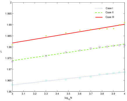
Figure 2: Impact of $m$ on $L$

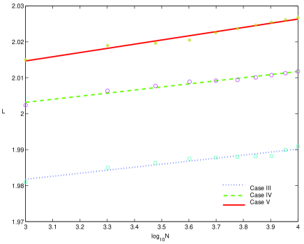
Figure 3: Impact of $p$ on $L$

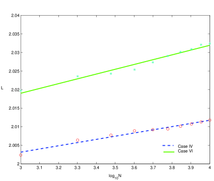
Figure 4: Impact of $\gamma$ on $L$

6 Conclusions and Discussions

There are two main contributions in this paper. First, by successfully integrating randomness and adaptability, we introduce a simple yet very flexible model for scale networks. While, as demonstrated in the previous sections, a number of the existing models are, in some way, special cases of our model, we are still able to derive an explicit expression for the network degree distribution. Our second contribution is the analytical expressions that we obtain for the clustering coefficient for a large class of scale-free networks. Apparently, there are not many successes in the literature for cluster coefficients due to analytical difficulties. Thus, the method we use in section 4 should be useful for others in the future.

Our discussion of cluster coefficients leads to an important observation, i.e., Remark 3 in section 4. Without hereditary, the important small world phenomenon displayed in real networks cannot be captured in our model as well as in many existing models. This shows much remain to be done in our quest to understand complex networks better.

Some attempts have been made in including hereditary. Ravasz and Barab$\acute{a}$si [21] build up a model of hierarchical organization with deterministic copy of a module. Dorogovtsev et al. [20] model scale-free networks by a deterministic pseudofractal graph. Although the authors show that the clustering coefficient of a node follows a power law with respect to the degree of the node, randomness and adaptability are absent. Solé et al. [22] investigate proteome growth model with random node duplications, old removal edges, and newly added edges. Empirically, they find by simulation that their model can explain the macroscopic features exhibited by the proteome. Klemm and Egu$\acute{\imath}$luz [23]’s model combines the motif copy and the BA model using a probability $\mu$. For $\mu=0$, their model has the characters of small-world networks. For $\mu=1$, their model is equivalent to the BA model. But, due to the analytical difficulty for $0<\mu<1$, the performance of the model can not be well studied. Holme and Kim [24] integrate preferential attachment with triad information to construct a scale-free network. By simulation, they show that their model can generate small-world characters.

References

- [1] R. Albert, A.-L. Barabsi, Statistical mechanics of complex networks, Rev. Mod. Phys. 74, 47 (2002).
- [2] S.H. Strogatz, Exploring complex networks, Nature 410, 268 (2001).
- [3] P. Erdös, A. Rényi, On the evolution of random graphs, Publ. Math. Inst. Hung. Acad. Sci. 5, 17 (1960).
- [4] D.J. Watts, S.H. Strogatz, Collective dynamics of small-world networks, Nature 393, 440 (1998).
- [5] R. Albert, H. Jeong, A.-L. Barabsi, Diameter of the world-wide web, Nature 401, 130 (1999).
- [6] A.-L. Barabsi, R. Albert, H. Jeong, Mean-field theory for scale-free random networks, Physica A 272, 173 (1999).
- [7] A.-L. Barabsi, R. Albert, Emergence of scaling in random networks, Science 286, 509 (1999).
- [8] P.L. Krapivsky, S. Redner, F. Leyvraz, Connectivity of growing random networks, Phys. Rev. Lett. 85, 4629 (2000).
- [9] S.N. Dorogovtsev, J.F.F. Mendes, A.N. Samukhin, Structure of growing networks with preferential linking, Phys. Rev. Lett. 85, 4633 (2000).
- [10] S.N. Dorogovtsev, J.F.F. Mendes, Scaling behaviour of developing and decaying networks, Europhys. Lett. 52, 33 (2000).
- [11] R. Albert, A.-L. Barabsi, Topology of evolving networks: Local events and universality, Phys. Rev. Lett. 85, 5234 (2000).
- [12] S.N. Dorogovtsev, J.F.F. Mendes, Evolution of networks with aging of sites, Phys. Rev. E 62, 1842 (2000).
- [13] P.L. Krapivsky, G.J. Rodgers, S. Redner, Degree distributions of growing networks, Phys. Rev. Lett. 86, 5401 (2001).
- [14] J.M. Kleinberg, R. Kumar, P. Raghavan, S. Rajagopalan, A. Tomkins, Proceedings of the th Annual International Conference, COCOON’, Tokyo, 1, 1999.
- [15] R. Kumar, P. Raghavan, S. Rajagopalan, D. Sivakumar, A. Tomkins,E. Upfal, The web as a graph, Proceedings of th symposium on Principles of Database systems, 1, 2000.
- [16] R. Kumar, P. Raghavan, S. Rajagopalan, D. Sivakumar, A. Tomkins,E. Upfal, Stochastic models for the web graph, Proceedings of th IEEE symposium on Foundations of Computer Science, 57, 2000.
- [17] P.L. Krapivsky, S. Redner, Organization of growing random networks, Phys. Rev. E. 63, 066123 (2001).
- [18] Z. Liu, Y. Lai, N. Ye, P. Dasgupta, Connectivity distribution and attack tolerance of general networks with both preferential and random attachments, Physics Letters A 303, 337 (2002).
- [19] Q. Chen, D. Shi, The modeling of scale-free networks, Physica A 335, 240 (2004).
- [20] S. Dorogovtsev, A. Goltsev2, J. Mendes, Pseudofractal scale-free web, Phys. Rev. E 65, 066122 (2002).
- [21] E. Ravasz, A.-L. Barabsi, Hierarchical organization in complex networks, Phys. Rev. E 67, 026112 (2003).
- [22] R. V. Solé, R. Pastor-Satorras1, E. D. Smith, T. Kepler, A model of large-scale proteome evolution, working paper, 2002.
- [23] K. Klemm, V. M. Eguluz, Growing scale-free networks with small-world behavior, Phys. Rev. E 65, 057102 (2002).
- [24] P. Holme, B. Kim, Growing scale-free networks with tunable clustering. Kim, Phys. Rev. E 65, 026107 (2002).