Size–Dependent Bruggeman Approach for Dielectric–Magnetic Composite Materials

Akhlesh Lakhtakia, Tom G. Mackay

Received Month 00, 2004.

A. Lakhtakia, CATMAS—Computational & Theoretical Materials Science Group, Department of Engineering Science & Mechanics, Pennsylvania State University, University Park, PA 16802–6812, USA.

E–mail: akhlesh@psu.edu

T.G. Mackay, School of Mathematics, University of Edinburgh,

Edinburgh EH9 3JZ, United Kingdom

E–mail: T.Mackay@ed.ac.uk

Correspondence to Mackay

Abstract Expressions arising from the Bruggeman approach for the homogenization of dielectric–magnetic composite materials, without ignoring the sizes of the spherical particles, are presented. These expressions exhibit the proper limit behavior. The incorporation of size dependence is directly responsible for the emergence of dielectric–magnetic coupling in the estimated relative permittivity and permeability of the homogenized composite material.

Keywords  Bruggeman approach, Dielectric–magnetic material, Homogenization, Maxwell Garnett approach, Particulate composite material, Size dependence

1 Introduction

The objective of this communication is to introduce a size–dependent variant of the celebrated Bruggeman approach [1, Eq. 32] and thereby couple the dielectric and magnetic properties of a particulate composite material (PCM) with isotropic dielectric–magnetic constituent materials.

Homogenization of PCMs has been a continuing theme in electromagnetism for about two centuries [2]. The most popular approaches consider the particles to be vanishingly small, point–like entities [3, 4]. Much of the literature is devoted to dielectric PCMs [3, 5], with application to magnetic PCMs following as a result of electromagnetic duality [6, Sec. 4-2.3]. When PCMs with both dielectric and magnetic properties are considered, no coupling arises between the two types of constitutive properties if the particles are vanishingly small. It is this coupling that has gained importance in the last few years, with the emergence of metamaterials [7].

Investigation of scattering literature quickly reveals that dielectric–magnetic coupling in PCMs emerges only when particles are explicitly taken to be of nonzero size [8, 9, 10], although the particle size must still be electrically small for the concept of homogenization to remain valid [2, p. xiii], [11]. To the best of our knowledge, available homogenization formulas for dielectric–magnetic PCMs that also account for dielectric–magnetic coupling are applicable only to dilute composites because they are set up using the Mossotti–Clausius approach (also called the Lorenz–Lorentz approach and the Maxwell Garnett approach [12]). Use of the Bruggeman approach is preferred, while maintaining the particle size as nonzero, for nondilute composites [12].

Accordingly, in Section 2 we apply the Bruggeman approach to derive size–dependent homogenization formulas for dielectric–magnetic PCMs comprising spherical particles. Sample results are discussed and conclusions are drawn therefrom in Section 3. An $\exp(-i\omega t)$ time–dependence is implicit, with $\omega$ being the angular frequency. The free–space (i.e., vacuum) wavenumber is denoted by $k_{0}$.

2 Theory

Let us consider a particulate composite material with $L$ constituent materials. The relative permittivity and the relative permeability of the $\ell$th constituent material, $\ell\in[1,\,L]$, are denoted respectively by $\epsilon_{\ell}$ and $\mu_{\ell}$, the radius of the spherical particles of that material is denoted by $R_{\ell}$, and the volumetric fraction by $f_{\ell}$. Clearly,

$$\sum_{\ell=1}^{L}\,f_{\ell}=1\,.$$ (1)

Our task is to estimate $\epsilon_{HCM}$ and $\mu_{HCM}$, which are the relative permittivity and the relative permeability of the homogenized composite material (HCM).

According to the Bruggeman approach [4, 10], the following two equations have to be solved:

$$\sum_{\ell=1}^{L}f_{\ell}\,\alpha^{\ell/Br}_{e}=0\,,\quad\sum_{\ell=1}^{L}f_{\ell}\,\alpha^{\ell/Br}_{h}=0\,.$$ (2)

Here, $\alpha_{e}^{a/b}$ and $\alpha_{h}^{a/b}$ are the polarizability density and the magnetizability density, respectively, of an electrically small sphere of material $a$ embedded in material $b$. In the limit of the particulate radius tending to zero, expressions of these two densities are available as follows [13]:

$$\left.\begin{array}[]{ll}\alpha_{e}^{a/b}=3\epsilon_{b}\frac{\epsilon_{a}-\epsilon_{b}}{\epsilon_{a}+2\epsilon_{b}}\\[5.0pt] \alpha_{h}^{a/b}=3\mu_{b}\frac{\mu_{a}-\mu_{b}}{\mu_{a}+2\mu_{b}}\end{array}\right\}\,.$$ (3)

However, when the sphere radius is nonzero, the foregoing expressions mutate to include both the radius $R_{a}$ of the embedded sphere and the refractive index

$$n_{b}=\sqrt{\epsilon_{b}\mu_{b}}$$ (4)

of the embedding material; thus [10]

$$\left.\begin{array}[]{ll}\alpha_{e}^{a/b}=3\epsilon_{b}\frac{\epsilon_{a}-\epsilon_{b}}{\epsilon_{a}(1-2\tau_{a/b})+2\epsilon_{b}(1+\tau_{a/b})}\\[5.0pt] \alpha_{h}^{a/b}=3\mu_{b}\frac{\mu_{a}-\mu_{b}}{\mu_{a}(1-2\tau_{a/b})+2\mu_{b}(1+\tau_{a/b})}\end{array}\right\}\,,$$ (5)

where

$$\tau_{a/b}=(1-ik_{0}R_{a}n_{b})\exp(ik_{0}R_{a}n_{b})-1\,.$$ (6)

More complicated expressions than (5) can be devised by using the Lorenz–Mie–Debye formulation for scattering by a sphere [8], but do not lead to significantly different results for electrically small spheres. In the limit $R_{a}\to 0$, expressions (5) reduce to (3) because

$$\lim_{R_{a}\to 0}\tau_{a/b}=0\,.$$ (7)

Clearly, the incorporation of particle size–dependence via (5) in (2) leads to a coupling of the relative permittivities and the relative permeabilities.

3 Results and Conclusion

In order to investigate the properties of (2), let us simplify it for a two–constituent composite material: $L=2$. Expressions (2) for the size–dependent Bruggeman approach then read as follows:

$$\left.\begin{array}[]{ll}0=f_{1}\frac{\epsilon_{1}-\epsilon_{Br}}{\epsilon_{1}(1-2\tau_{1/Br})+2\epsilon_{Br}(1+\tau_{1/Br})}\\[5.0pt] \quad+\,(1-f_{1})\frac{\epsilon_{2}-\epsilon_{Br}}{\epsilon_{2}(1-2\tau_{2/Br})+2\epsilon_{Br}(1+\tau_{2/Br})}\\[8.0pt] 0=f_{1}\frac{\mu_{1}-\mu_{Br}}{\epsilon_{1}(1-2\tau_{1/Br})+2\mu_{Br}(1+\tau_{1/Br})}\\[5.0pt] \quad+\,(1-f_{1})\frac{\mu_{2}-\mu_{Br}}{\mu_{2}(1-2\tau_{2/Br})+2\mu_{Br}(1+\tau_{2/Br})}\end{array}\right\}\,.$$ (8)

These two coupled equations have to be solved together in order to obtain the estimates $\epsilon_{Br}$ and $\mu_{Br}$ of $\epsilon_{HCM}$ and $\mu_{HCM}$ as functions of $k_{0}$, $f_{1}$, $R_{1}$ and $R_{2}$.

Equations (8) have to be solved iteratively, and the Newton–Raphson method is very useful for that purpose [14, Sec. 6.5.2]. Typically, this method requires an initial guess, which can be supplied using the Maxwell Garnett approach [2, 3]. If $f_{1}>f_{2}$, then material $1$ should be treated as the host material while material $2$ is dispersed in particulate form; and the size–dependent Maxwell Garnett estimates of $\epsilon_{HCM}$ and $\mu_{HCM}$ are then obtained as follows:

$$\left.\begin{array}[]{ll}\epsilon_{MG,1}=\epsilon_{1}+(1-f_{1})\frac{\alpha_{e}^{2/1}}{1-(1-f_{1})\frac{\alpha_{e}^{2/1}}{3\epsilon_{1}}}\\[5.0pt] \mu_{MG,1}=\mu_{1}+(1-f_{1})\frac{\alpha_{h}^{2/1}}{1-(1-f_{1})\frac{\alpha_{h}^{2/1}}{3\mu_{1}}}\end{array}\right\}\,.$$ (9)

On the other hand, the size–dependent Maxwell Garnett estimates

$$\left.\begin{array}[]{ll}\epsilon_{MG,2}=\epsilon_{2}+f_{1}\frac{\alpha_{e}^{1/2}}{1-f_{1}\frac{\alpha_{e}^{1/2}}{3\epsilon_{2}}}\\[5.0pt] \mu_{MG,2}=\mu_{2}+f_{1}\frac{\alpha_{h}^{1/2}}{1-f_{1}\frac{\alpha_{h}^{1/2}}{3\mu_{2}}}\end{array}\right\}\,$$ (10)

appear more appropriate when $f_{2}>f_{1}$. Incorporation of size dependence couples dielectric and magnetic properties also in (9) and (10).

Let us note that the limits

$$\left.\begin{array}[]{ll}\lim_{f_{1}\to 0}\left[\begin{array}[]{l}\epsilon_{Br}\\ \mu_{Br}\end{array}\right]=\left[\begin{array}[]{l}\epsilon_{2}\\ \mu_{2}\end{array}\right]\\[7.0pt] \lim_{f_{1}\to 1}\left[\begin{array}[]{l}\epsilon_{Br}\\ \mu_{Br}\end{array}\right]=\left[\begin{array}[]{l}\epsilon_{1}\\ \mu_{1}\end{array}\right]\end{array}\right\}\,$$ (11)

satisfied by the solutions of (8) are physically correct, and are not affected by the incorporation of size dependence in the Bruggeman approach. In contrast, the size–dependent Maxwell Garnett expressions (9) and (10) do not exhibit physically reasonable limits when the host material vanishes; i.e.,

$$\left.\begin{array}[]{ll}\lim_{f_{1}\to 0}\left[\begin{array}[]{l}\epsilon_{MG,1}\\ \mu_{MG,1}\end{array}\right]\neq\left[\begin{array}[]{l}\epsilon_{2}\\ \mu_{2}\end{array}\right]\,,&\quad{\rm if}\,R_{2}\neq 0\\[7.0pt] \lim_{f_{1}\to 0}\left[\begin{array}[]{l}\epsilon_{MG,1}\\ \mu_{MG,1}\end{array}\right]=\left[\begin{array}[]{l}\epsilon_{2}\\ \mu_{2}\end{array}\right]\,,&\quad{\rm if}\,R_{2}=0\\[7.0pt] \lim_{f_{1}\to 1}\left[\begin{array}[]{l}\epsilon_{MG,1}\\ \mu_{MG,1}\end{array}\right]=\left[\begin{array}[]{l}\epsilon_{1}\\ \mu_{1}\end{array}\right]\end{array}\right\}\,,$$ (12)

and analogously for $\epsilon_{MG,2}$ and $\mu_{MG,2}$. The foregoing limits are borne out by the plots of $\epsilon_{HCM}$ and $\mu_{HCM}$ versus $f_{1}$ presented in Figures 1–3.

Figure 1 presents estimates of the real and imaginary parts of the relative permittivity and the relative permeability of the HCM when $\epsilon_{1}=1.5$, $\mu_{1}=1$, $\epsilon_{2}=5+i0.2$, and $\mu_{2}=2+i0.1$, and the sizes $R_{1}=R_{2}=0$. Calculations for the relative permittivity and the relative permeability then decouple from each other.

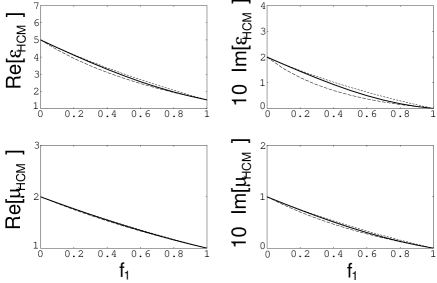
Fig. 1: Estimates of the real and imaginary parts of the relative permittivity and the relative permeability of a homogenized composite material (HCM) with two constituent materials ($\epsilon_{1}=1.5$, $\mu_{1}=1$, $\epsilon_{2}=5+i0.2$, and $\mu_{2}=2+i0.1$) as functions of the volumetric fraction $f_{1}=1-f_{2}$. Size–independent Maxwell Garnett approach with material $1$ as the host material (dashed line); Size–independent Maxwell Garnett approach with material $2$ as the host material (dotted line); Size–independent Bruggeman approach (solid line). $k_{0}R_{1}=k_{0}R_{2}=0$.

The analogous plots in Figure 2 were drawn for $R_{1}=R_{2}\neq 0$. These plots are quite different from those in the preceding figure. The imaginary parts of $\epsilon_{HCM}$ and $\mu_{HCM}$ appear to be more affected by the size dependence than the real parts. Indeed, were both constituent materials totally nondissipative, the imaginary parts of $\tau_{a/b}$–terms would still give rise to imaginary parts of both $\epsilon_{HCM}$ and $\mu_{HCM}$ [12]. We also conclude from comparing Figures 1 and 2 that dielectric–magnetic coupling proportionally affects the imaginary parts of the HCM constitutive parameters more than their real parts.

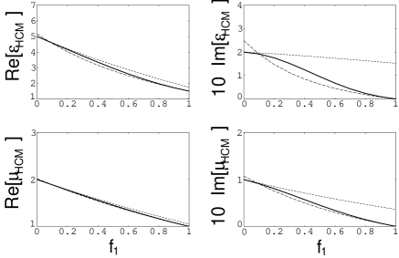
Fig. 2: Estimates of the real and imaginary parts of the relative permittivity and the relative permeability of a homogenized composite material (HCM) with two constituent materials ($\epsilon_{1}=1.5$, $\mu_{1}=1$, $\epsilon_{2}=5+i0.2$, and $\mu_{2}=2+i0.1$) as functions of the volume fraction $f_{1}=1-f_{2}$. Size–dependent Maxwell Garnett approach with material $1$ as the host material (dashed line); Size–dependent Maxwell Garnett approach with material $2$ as the host material (dotted line); Size–dependent Bruggeman approach (solid line). $k_{0}R_{1}=k_{0}R_{2}=0.2$.

There is no reason for the particles of both constituent materials to be of the same size (or have the same distribution of size, in general). The plots in Figure 3 were drawn for $R_{2}=3R_{1}$. Clearly from this figure and Figure 2, the effect of different particle sizes on dielectric–magnetic coupling can be substantial.

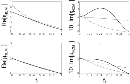
Fig. 3: Same as Figure 2, except that $k_{0}R_{1}=0.2$ and $k_{0}R_{2}=0.6$.

The permeability contrast between the two constituent materials chosen for Figures 1–3 is less than the permittivity contrast. We notice that the effect of size dependence on $\mu_{HCM}$ is less than on $\epsilon_{HCM}$. This implies that dielectric–magnetic coupling affects the more contrasting constitutive parameter more.

To conclude, we have here implemented the Bruggeman approach for the homogenization of dielectric–magnetic composite materials, without ignoring the sizes of the spherical particles. These expressions exhibit the proper limit behavior. The incorporation of size dependence is directly responsible for the emergence of dielectric–magnetic coupling in the estimated relative permittivity and permeability of the homogenized composite material. The size–dependent Bruggeman estimates are compared with the size–dependent Maxwell Garnet estimates, which do not necessarily evince the proper limit behavior and are therefore applicable to dilute composite materials.

Akhlesh Lakhtakia  was born in Lucknow, India, in 1957. Presently, he is a Distinguished Professor of Engineering Science and Mechanics at the Pennsylania State University. He is a Fellow of the Optical Society of America, SPIE–The International Society for Optical Engineering, and the Institute of Physics (United Kingdom). He has either authored or co–authored about 650 journal papers and conference publications, and has lectured on waves and complex mediums in many countries. His current research interests lie in the electromagnetics of complex mediums, sculptured thin films, and nanotechnology. For more information on his activities, please visit his website: www.esm.psu.edu/$\sim$axl4/

Tom G. Mackay  graduated MSci in Mathematics from the University of Glasgow, UK, in 1998, after spending the previous ten years working as a bioengineer at Glasgow Royal Infirmary. He spent the next three years engaged in postgraduate studies in the Department of Mathematics at the University of Glasgow, under the supervision of Prof. Werner S. Weiglhofer. Upon completing his PhD thesis in 2001, he moved to the University of Edinburgh, UK, where he is currently employed as a lecturer in the School of Mathematics. His research interests are primarily related to the homogenization of complex electromagnetic systems. He is also interested in biological applications of electromagnetic theory.

References

- [1] Bruggeman, D.A.G.: Berechnung verschiedener physikalischer Konstanten von heterogenen Substanzen. I. Dielektrizitätskonstanten und Leitfähigkeiten der Mischkörper aus isotropen Substanzen. Ann. Phys. Lpz. 24 (1935), 636–679.
- [2] Lakhtakia, A. (ed): Selected Papers on Linear Optical Composite Materials. Bellingham, WA, USA: SPIE Press, 1996.
- [3] Neelakanta, P.S.: Handbook of Electromagnetic Materials. Boca Raton, FL, USA: CRC Press, 1995.
- [4] Michel, B.: Recent developments in the homogenization of linear bianisotropic composite materials. In: Singh, O.N.; Lakhtakia, A. (eds): Electromagnetic Fields in Unconventional Materials and Structures. New York, NY, USA: Wiley, 2000.
- [5] Ward, L.: The Optical Constants of Bulk Materials and Films. Bristol, United Kingdom: Adam Hilger, 1988.
- [6] Lakhtakia, A.: Beltrami Fields in Chiral Media. Singapore: World Scientific, 1994.
- [7] Walser, R.M.: Metamaterials: An introduction. In: Weiglhofer, W.S.; Lakhtakia, A. (eds): Introduction to Complex Mediums for Optics and Electromagnetics. Bellingham, WA, USA: SPIE Press, 2003.
- [8] Grimes, C.A.: Electromagnetic properties of random material. Waves Random Media 1 (1991), 265–273.
- [9] Grimes, C.A.: Calculation of the effective electromagnetic properties of granular materials. In: Lakhtakia, A. (ed): Essays on the Formal Aspects of Electromagnetic Theory. Singapore: World Scientific, 1993.
- [10] Lakhtakia, A., Shanker, B.: Beltrami fields within continuous source regions, volume integral equations, scattering algorithms and the extended Maxwell–Garnett model. Int. J. Appl. Electromag. Mater. 4 (1993), 65–82.
- [11] Lorenz, L.V.: Experimentale og theoretiske unders gelser over legemernes brydningsforhold, II. K. Dan. Vidensk. Selsk. Forh. 10 (1875), 485–518.
- [12] Prinkey, M.T.; Lakhtakia, A.; Shanker, B.: On the Extended Maxwell–Garnett and the Extended Bruggeman approaches for dielectric–in–dielectric composites. Optik 96 (1994), 25–30.
- [13] Lakhtakia, A.; Varadan, V.K.; Varadan, V.V.: Dilute random distribution of small chiral spheres. Appl. Opt. 29 (1990), 3627–3632.
- [14] Chapra, S.C.; Canale, R.P.: Numerical Methods for Engineers, 4th ed. New York, NY, USA: McGraw–Hill, 2002.